Estimation and inference for a regression model depend on several assumptions. The three main categories of assumptions are:

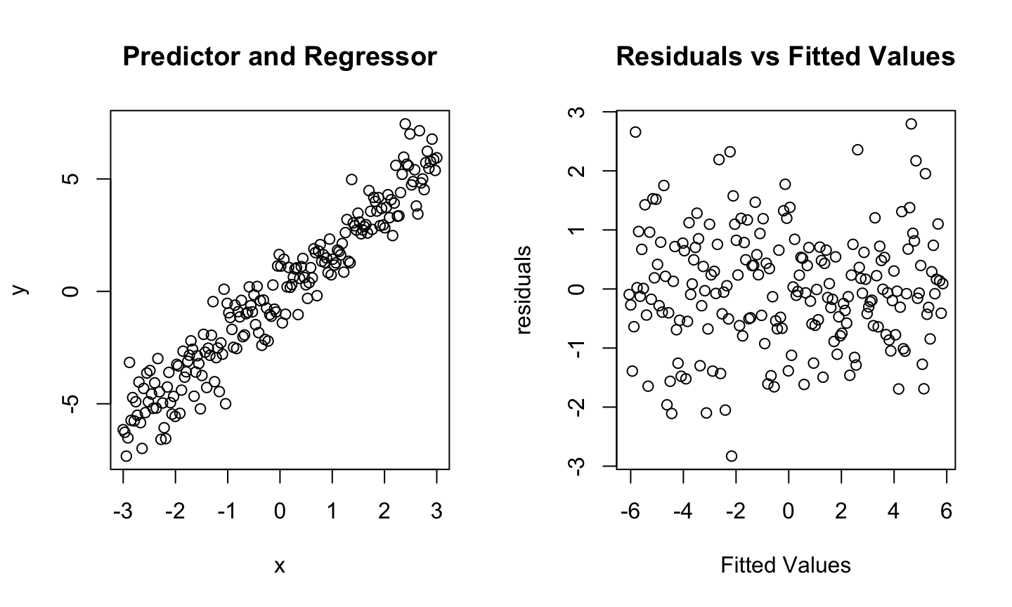
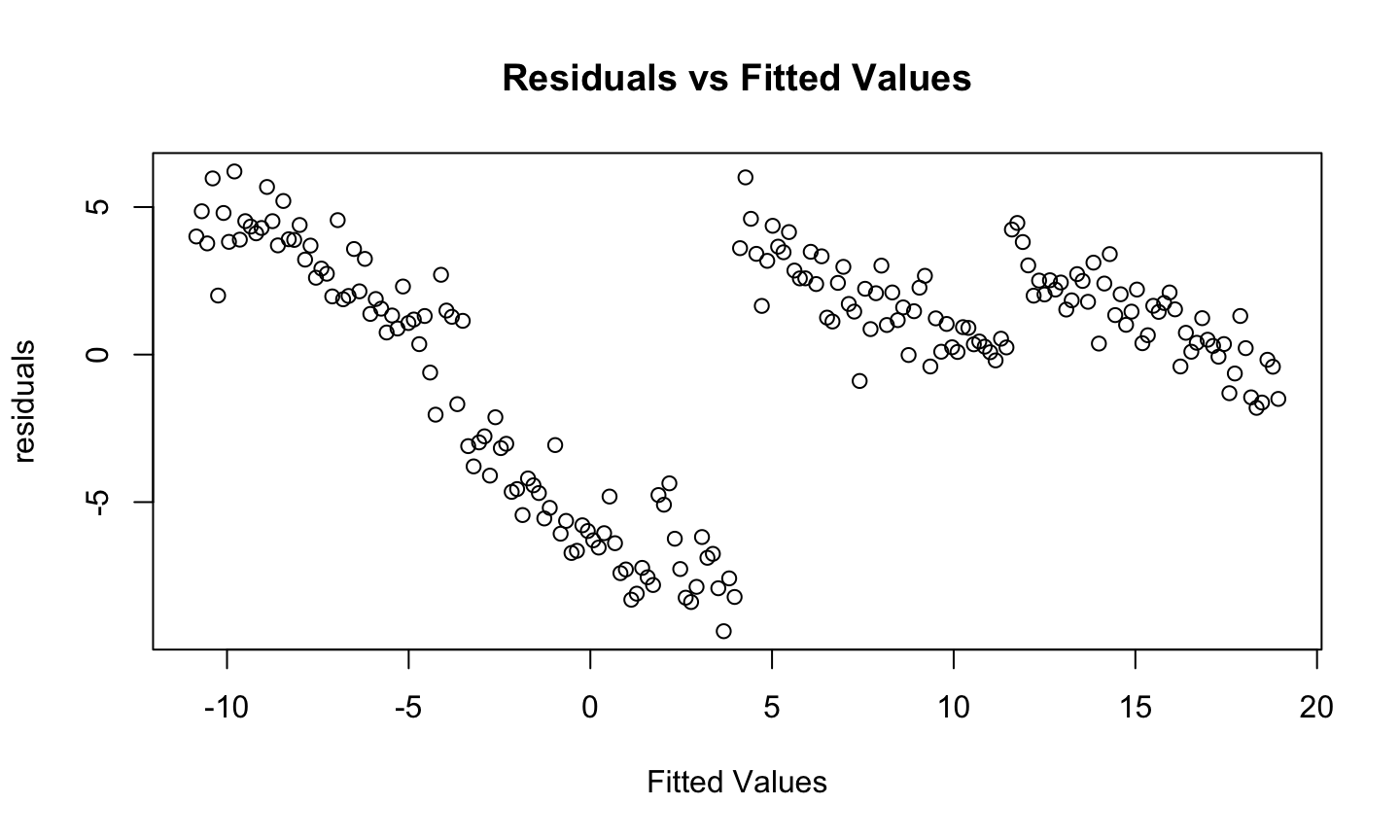
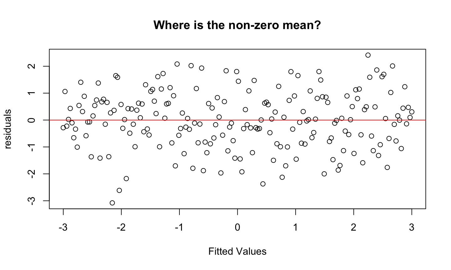
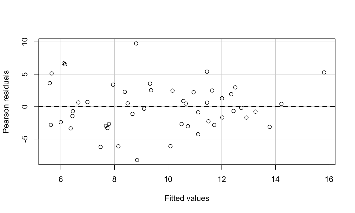
Model: The structural (mean) part of the model is correct, i.e., \(E(y)=X\beta\).

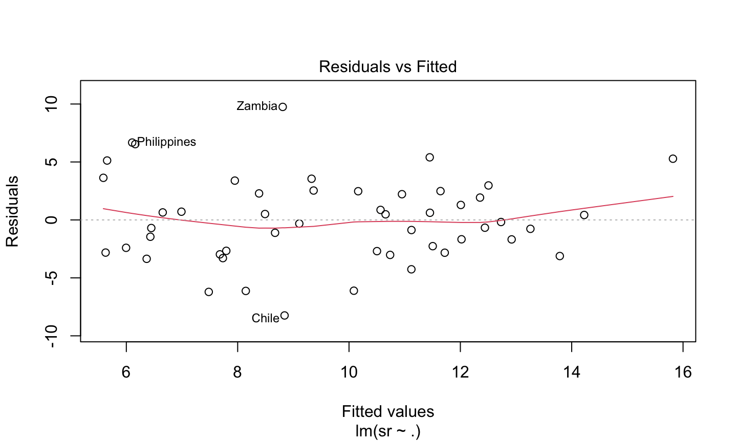
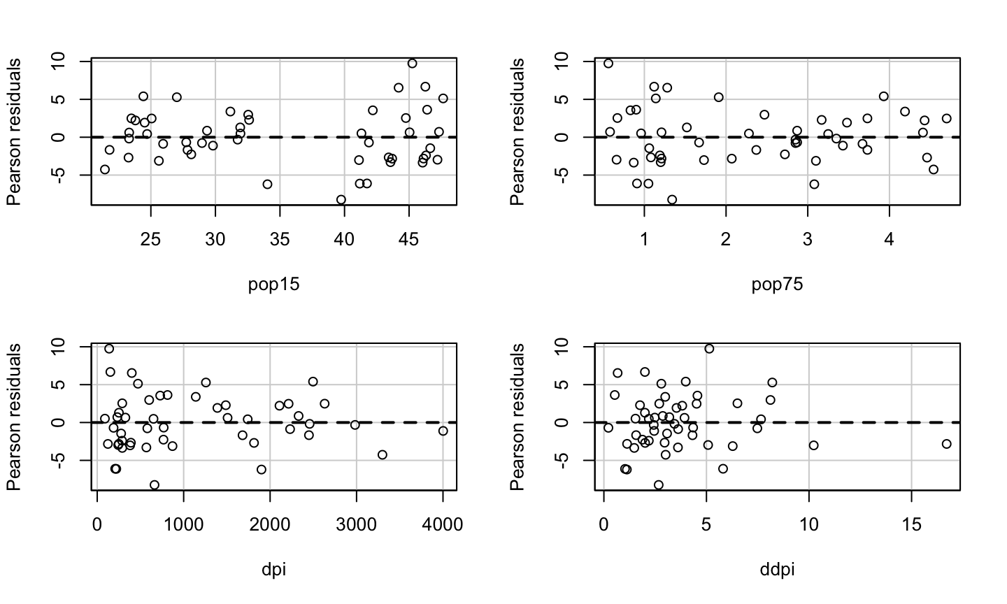
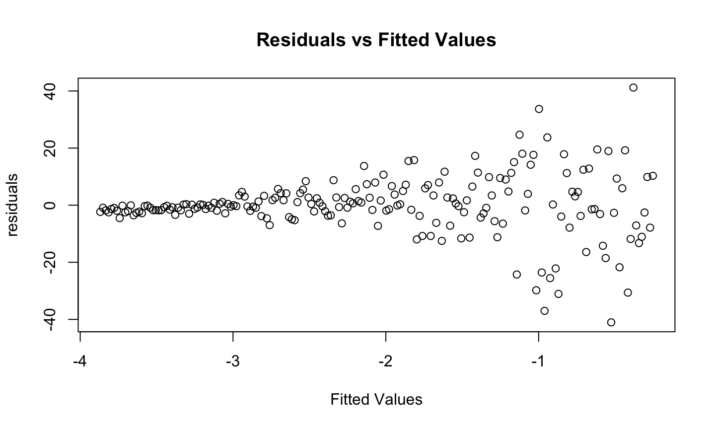
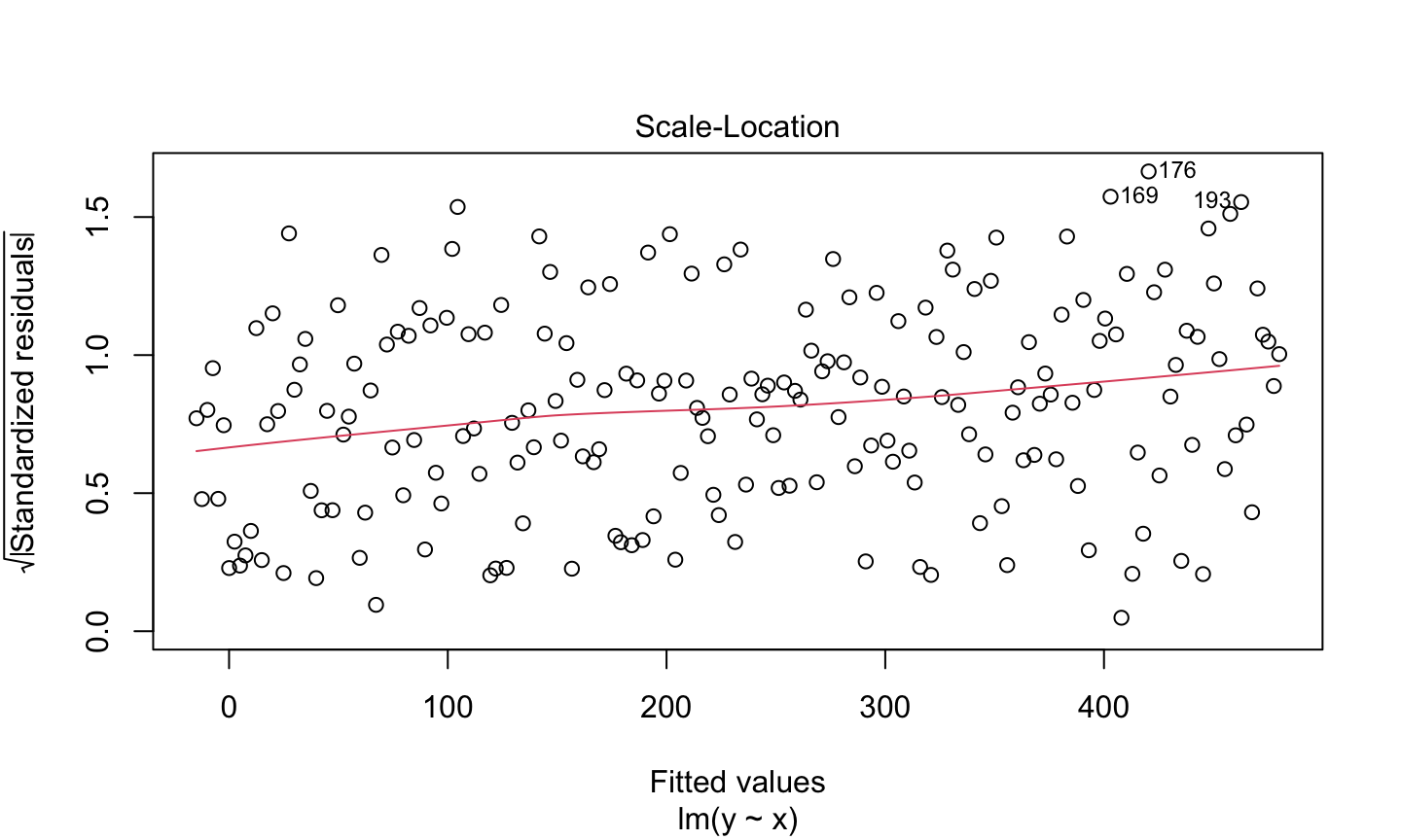
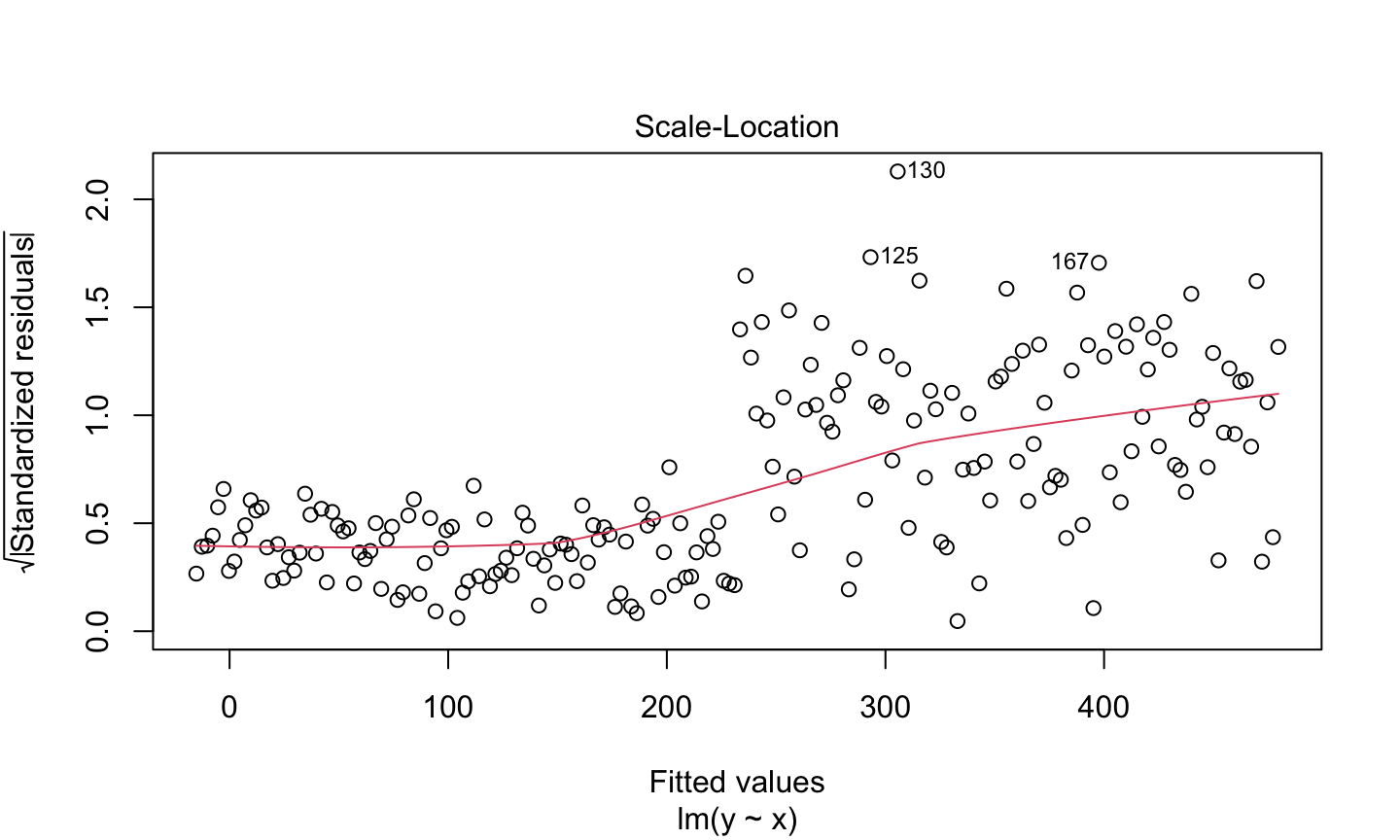
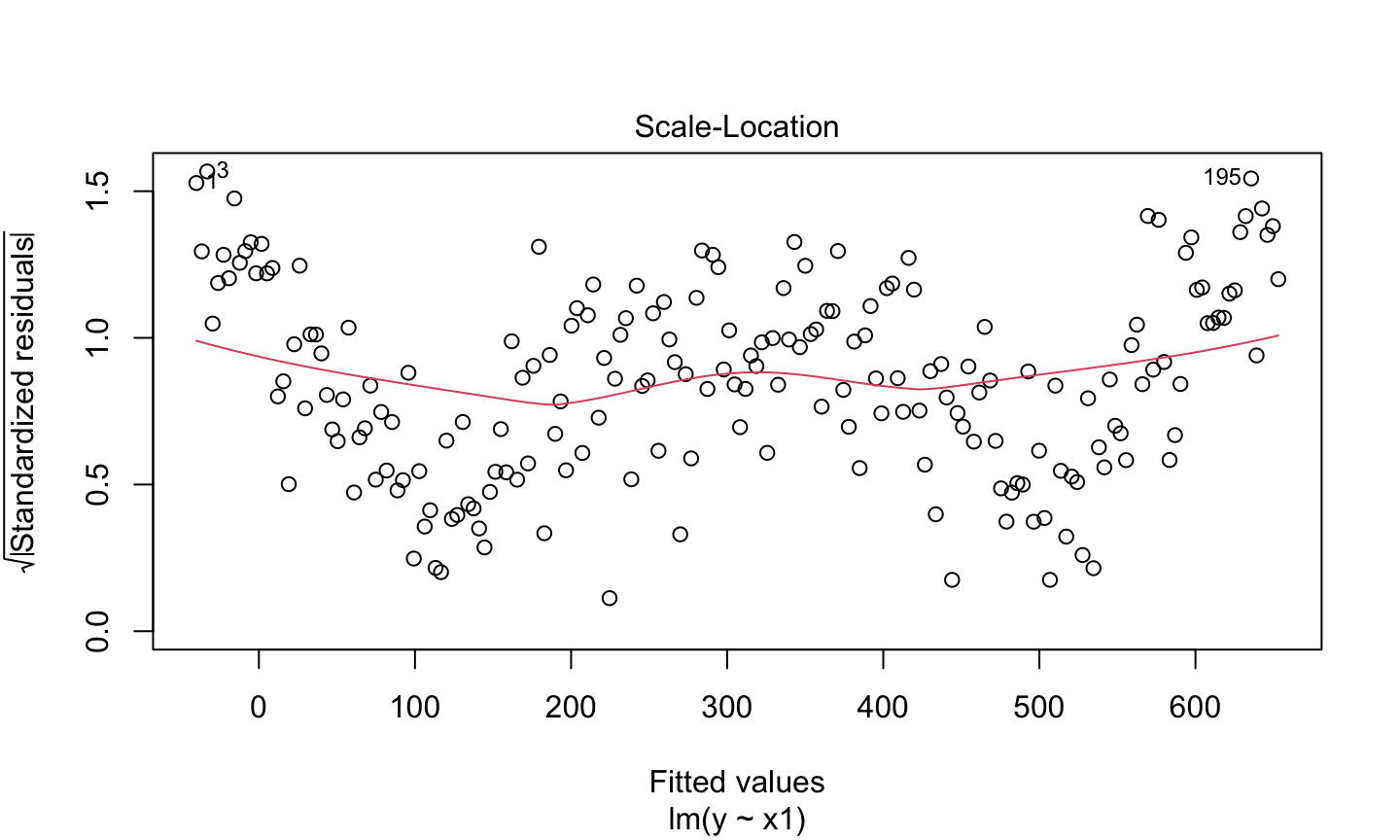
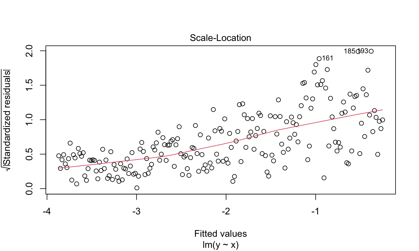
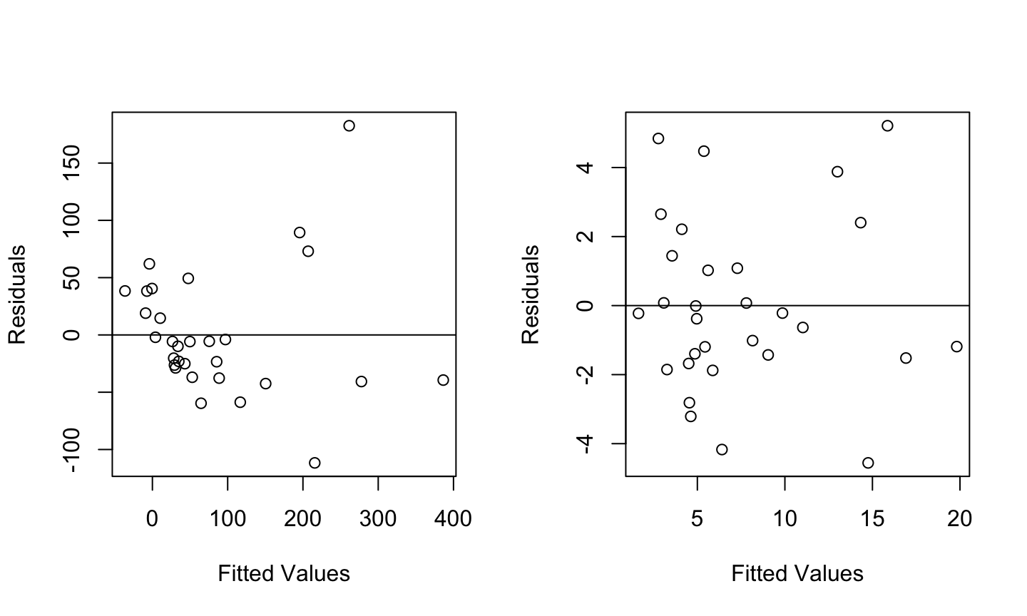
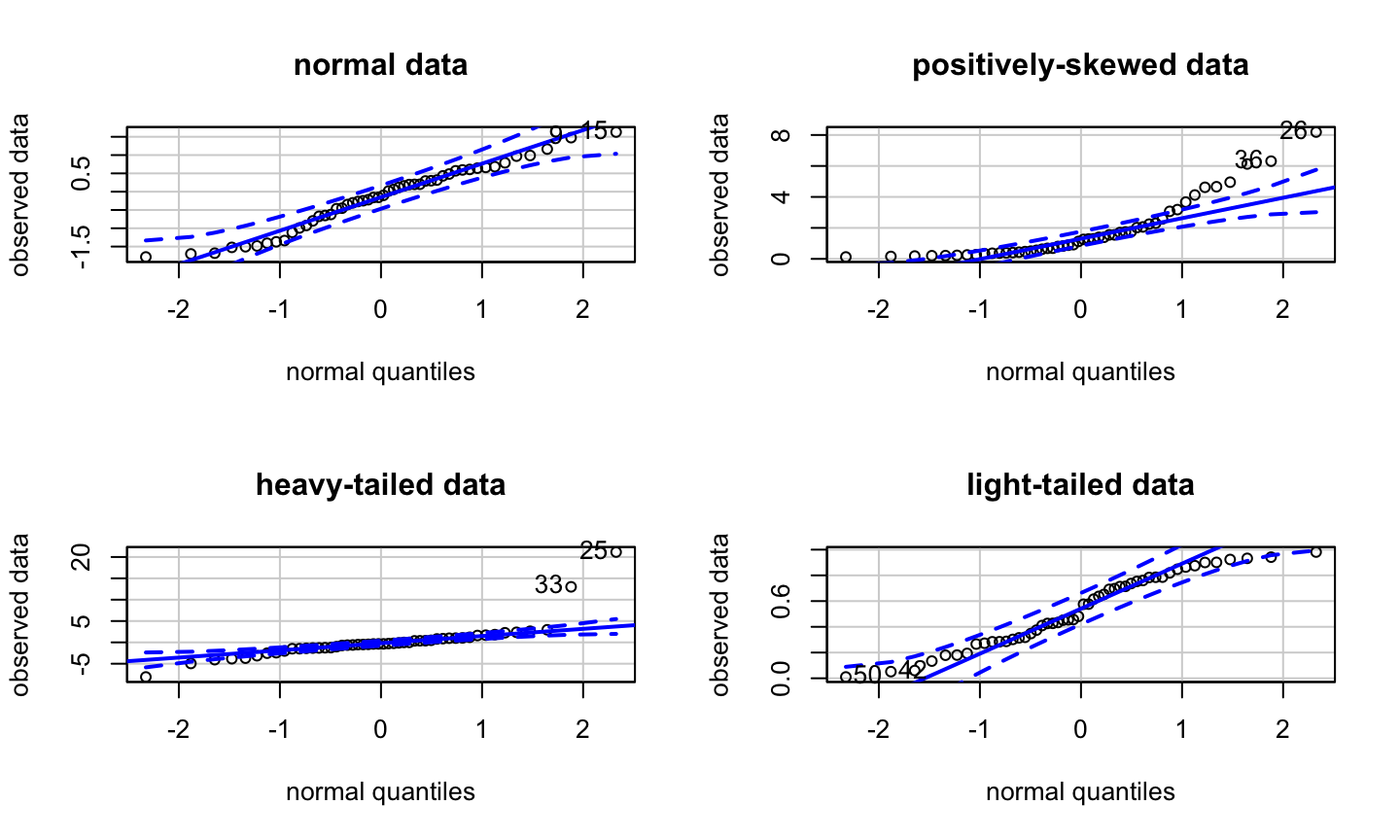
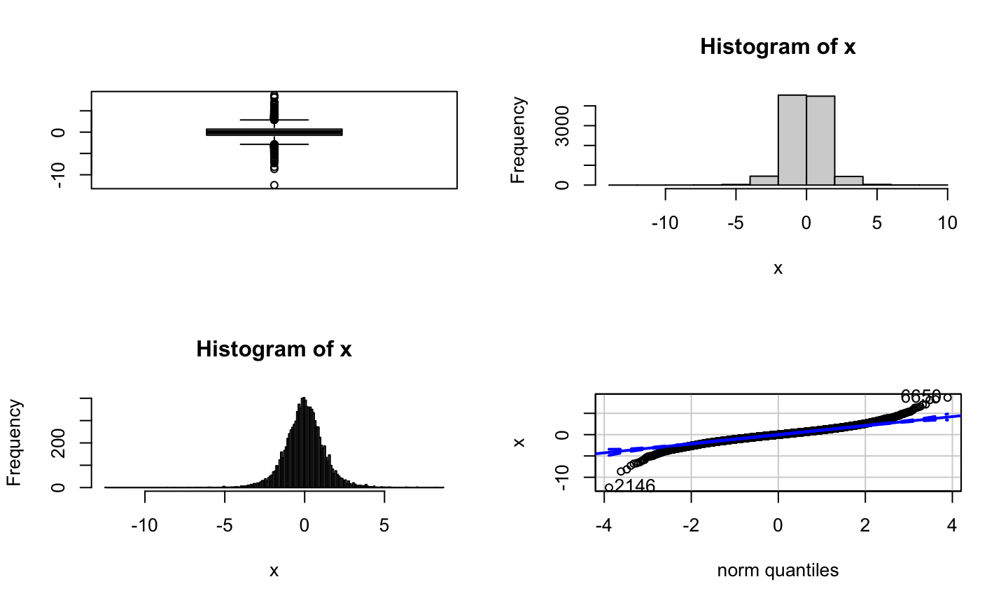
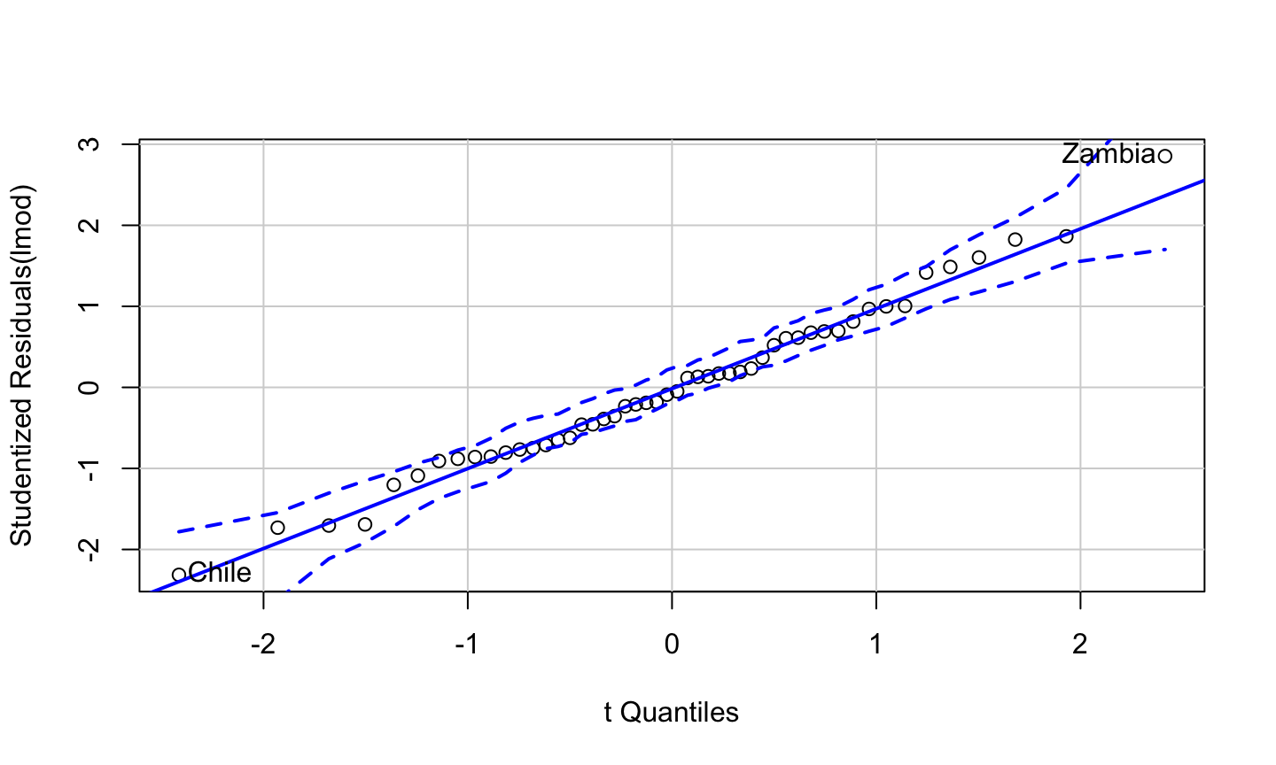
Error: \(\epsilon\sim N(0,\sigma^2 I)\), i.e., that the errors are normally distributed, independent, and identically distributed with mean 0 and variance \(\sigma^2\).

Unusual observations: All observations should be equally reliable and have approximately equal role in determining the regression results and in influencing conclusions.

Assumptions for \(\epsilon\) are tricky to check because \(\epsilon\) is not observed.

Assumptions for \(\epsilon\) allow us to derive expected properties for our residuals, \(\hat{\epsilon}\).

• The residuals are NOT interchangeable with the errors and have different properties.

Assumptions for ϵ are checked using \(\hat{\epsilon}\).

• If the observed residual behavior doesn’t match the expected behavior, we believe this was caused by a violation of the relevant error assumption.

• If \(E(\epsilon)=0\), then \(E(\hat{\epsilon}) = 0.\)
• If \(var(\epsilon)=\sigma^2 I\), i.e., the errors are uncorrected and have constatn variance, then \(var(\hat{\epsilon}) = \sigma^2(I-H)\), where \(H = X(X^TX)^{-1}X^T\) is the hat matrix.
• If \(E(\epsilon)=0\) and \(var(\epsilon)=\sigma^2I\), then \(cov(\hat{\epsilon}, \hat{y})=0_{n\times n}.\)
• If \(x_i\) is the \(i\)th regressor, then \(cov(\hat{\epsilon}, x_i)=0\).
• If an intercept is included in the fitted model, then \(\sum \hat{\epsilon}_i=0\).

The mean zero assumption means that the average deviation of each error from the true regression model is zero.

• Since we only observe a single value for each residual, we assess this assumption using the set of all residuals.

If the mean-zero error assumption is reasonable, then a plot of \(\hat{\epsilon}\) versus \(\hat{y}\) or \(\hat{\epsilon}\) versus \(x_i\) should be approximately symmetric around zero.

• This check implicitly assumes \(E(y)=X\beta\) and the errors are uncorrelated.

If the mean-zero error assumption is violated, then a plot of \(\hat{\epsilon}\) versus \(\hat{y}\) or \(x_i\) will have a systematic, asymmetrical pattern deviating from zero.

x <- seq(-3,3,length.out = 200)
y<-c()
y[1:50] <- 2*x[1:50] + rnorm(50)
y[51:100] <- 2*x[51:100] + rnorm(50, mean = -4)
y[101:150] <- 2*x[101:150] + rnorm(50, mean = 8)
y[151:200] <- 2*x[151:200] + rnorm(50, mean =12)
lmod = lm(y~x)
plot(lmod$residuals ~ lmod$fitted.values, main = 'Residuals vs Fitted Values', xlab = 'Fitted Values', ylab ='residuals')

x <- seq(-3,3,length.out = 200)
y <- 2*x + rnorm(200, mean = 500)
lmod = lm(y~x)
plot(lmod$residuals ~ x, main = 'Where is the non-zero mean?', xlab = 'Fitted Values', ylab ='residuals')
abline(0,0,col='red')

If a violation is detected, then you need to correct the structure of your model.

• This may include transforming the response or predictors in the model.
• This may include adding or deleting predictors from the model.
• You may need to consider more advanced forms of regression.

If the fitted R model is lmod:

• car::residualPlot(lmod) constructs a plot of \(\hat{\epsilon}\) versus \(\hat{y}\).
• car::residualPlots(lmod) constructs plots of \(\hat{\epsilon}\) versus \(\hat{y}\) each each predictor.
• plot(lmod, which = 1) construct a plot of \(\hat{\epsilon}\) versus \(\hat{y}\).

The savings data frame in the faraway package includes 5 savings-related variables in 50 countries averaged over the period 1960-1970:

• sr - savings rate. Personal saving divided by disposable income
• pop15 – percentage of population under age of 15
• pop75 – percentage of population over age of 75
• dpi - per-capita disposable income in dollars
• ddpi - percent growth rate of dpi

Is the mean-zero error assumption reasonable for the model regressing sr on the other four variables?

data(savings, package = "faraway")
lmod = lm(sr ~ ., data = savings)
library(car)

residualPlot(lmod, quadratic = FALSE)

plot(lmod, which = 1)

residualPlots(lmod, quadratic = FALSE, fitted = FALSE, tests = FALSE)

x<-seq(1,100,length.out = 200)
y <- 5*x -20 + rnorm(200)
plot(lm(y~x), which = 3)

x<-seq(1,100,length.out = 200)
y <- 5*x -20
y = y + c(rnorm(100,0, 1), rnorm(100, 0, 10))
lmod1 = lm(y~x)
plot(lmod1, which = 3)

x1 <- seq(1,100, length.out = 200)
x2 <- seq(1, 10, length.out = 200)
y <- 5*x1 + 2*x2^2 - 20 + rnorm(200, 0, 5)
plot(lm(y~x1), which = 3)

The constant variance assumption means that the average squared deviation of each error from the true regression model should be the same for every observation.

• Since we only observe a single value for each residual, we assess this assumption using the set of all residuals.

If the constant error variance assumption is correct, then a plot of ϵ ̂ versus y ̂ or x_i should be a random scatter of points and the spread of the residuals should have a constant thickness as you move from left to right along the x-axis of the plot.

• This check implicitly assumes the errors are uncorrelated.

If the constant error variance assumption is violated, then a plot of \(\hat{\epsilon}\) versus \(\hat{y}\) or \(x_i\) will have a systematic, varying spread of the residuals.

plot(lmod, which = 3)

If the non-constant error variance assumption is violated you should:

• Transformation of the response and/or predictors.

  • Square root and \(\log(y+c)\) transformations are common.
  • Transfomation of variables also correct for issues with model structure

• Consider fitting a weighted least squares (WLS) regression model instead of OLS.

  • Specially when the structure is approximately correct
  • Example : when measurement error of the response depends on the response variable

Left figure: Species ~ .

Right figure : $\sqrt{Species}$ ~ .

x1 = seq(1,100,length.out = 200)
y <- 5*x - 20 + rnorm(200) # Error for factor other than measurement 
y <- y + rnorm(200, 0, y^2/10) # Measurement error increase with y
plot(x1,y)

Use WLS.

par(mfrow = c(1,2))
data(savings,package="faraway")
lmod <- lm(sr ~ pop15+pop75+dpi+ddpi,savings)
plot(fitted(lmod),residuals(lmod),xlab="Fitted",ylab="Residuals")
abline(h=0)
plot(fitted(lmod),sqrt(abs(residuals(lmod))), xlab="Fitted",ylab=
    expression(sqrt(hat(epsilon))))

Suppose we have samples from two populations (\(Y = \{y_1,\dots y_n\}\) and \(T = \{t_1, \dots t_m\}\)). We can test if the variances \(\sigma_Y^2\) and \(\sigma_T^2\) are equal.

• Test statistic

\[\frac{S_Y^2}{S_T^2}\]

• Distribution

The test statistic follows a \(F(n-1,m-1)\) distribution.

par(mfrow = c(1,2))
plot(savings$pop15,residuals(lmod), xlab="Population under 15",ylab
="Residuals")
abline(h=0)
plot(savings$pop75,residuals(lmod), xlab="Population over 75",ylab ="Residuals")
abline(h=0)

sample1 = residuals(lmod)[savings$pop15>35]
sample2 = residuals(lmod)[savings$pop15<35]
var.test(sample1, sample2)

## 
##  F test to compare two variances
## 
## data:  sample1 and sample2
## F = 2.7851, num df = 22, denom df = 26, p-value = 0.01358
## alternative hypothesis: true ratio of variances is not equal to 1
## 95 percent confidence interval:
##  1.240967 6.430238
## sample estimates:
## ratio of variances 
##           2.785067

A q-q plot (quantile-quantile plot) of the residuals can be used to assess the assumption of normal errors.

• A q-q plot compares the residuals to “ideal” observations from a normal distribution.

• The sorted residuals are plotted against \(\phi^{-1}\left(\frac{i}{n+1}\right)\) for \(i=1,2,\dots ,n\), where \(\phi^{-1}\) is the inverse cdf (quantile) function of a standard normal distribution.

• If the residuals are distributed similarly to observations coming from a normal distribution, then the points of a q-q plot will lie approximately in a straight line at a 45 degree angle.

Histograms and boxplots are not as useful for checking normality as a q-q plot.

• Boxplots can obscure a lot of information.
• The shape of a histogram strongly depends on the number and size of the bins.

A formal test of normality can be performed using the Shapiro-Wilk test.

• The null hypothesis of the Shapiro-Wilk test is that the residuals are a random sample from a normal distribution.
  
• The alternative is that the residuals are not a sample from a normal distribution.
• A statistical decision is made using the usual approach with p-values.

While the Shapiro-Wilk test is a tidy way to assess normality, it is not as flexible as the q-q plot.

• It also does not suggest a way to correct the problem.
• It is easily influenced by the number of observations so that even minor departures from normality are detected, even when there is little reason to abandon the least squares approach.

• Estimates will still be unbiased (assuming the model is correct and the error mean is zero).
• Tests and confidence intervals will not be exact, but the central limit theorem says that the intervals and tests will be increasingly accurate as the sample size increases.
• The consequences can generally be ignored for short-tailed distributions.
• For skewed errors, a transformation may solve the problem.
• For heavy-tailed errors, it is best to use robust methods that give less weight to outlying observations.
• You may consider a different model. The problem may not be present in a different model.

qqPlot(lmod)

##  Chile Zambia 
##      7     46

shapiro.test(residuals(lmod))

## 
##  Shapiro-Wilk normality test
## 
## data:  residuals(lmod)
## W = 0.98698, p-value = 0.8524

It is difficult to check for correlated errors because there are so many possible patterns of correlation that may occur.

• The structure of temporal or spatial data make this easier to check.

If the errors are uncorrelated, then the residuals are typically close to uncorrelated.

A plot of \(\hat{\epsilon}\) versus time should be a random scatter of points if the errors are uncorrelated.

• Correlation among the errors is suggested when these plots have a clear pattern, e.g., lots of positive or negative residuals strung together or strings of residuals with alternating signs.

A plot of \(\hat{\epsilon}_{i+1}\) versus \(\hat{\epsilon}_i\) for \(i=1,\dots,n-1\), should be a random scatter of points if the errors are uncorrelated.

• If the errors are positively correlated, we expect this plot to have a positive slope among the points.
• If the errors are negatively correlated, we expect this plot to have a negative slope among the points.

The issue of global warming has attracted significant interest in recent years. Reliable records of annual temperatures taken with thermometers are only available back to the 1850s. Information about temperatures prior to this can be extracted from proxies such as tree rings. We can build a linear model to predict temperature since 1856 and then subsequently use this to predict earlier temperatures based on proxy information. The data we use here are included in the globwarm data set in the faraway package. The data are derived from Jones and Mann (2004).

Consider a model of temperature regressed on eight proxies.

• There are some missing values for nhtemp prior to 1856, so these observations are (automatically) omitted (by R) from our model.

• We then plot the residuals vs time.

data(globwarm,package="faraway")
lmod = lm(nhtemp ~ wusa + jasper + westgreen +
          chesapeake + tornetrask + urals + 
          mongolia + tasman, data = globwarm)

plot(residuals(lmod) ~ year, 
     data = na.omit(globwarm), ylab = "residuals")
abline(h = 0)

If the errors are uncorrelated, we expect a random scatter of points around \(\hat{\epsilon}=0\), which is certainly not the case here.

The cyclical pattern suggests positive serial correlation.

• Another approach to check for serial correlation is to plot successive pairs of residuals.

n = nobs(lmod)
plot(tail(residuals(lmod), n - 1) ~ 
     head(residuals(lmod), n - 1), 
     xlab = expression(hat(epsilon)[i]),
     ylab =expression(hat(epsilon)[i+1]))
abline(h= 0 , v = 0, col = grey(0.75))

The positive linear trend in the previous plot suggests positive serial correlation.

A formal test of serial correlation between residuals is the Durbin-Watson test. The Durbin-Watson test decides between:

\[H_0:\ \rho=0 \text{ versus } H_a:\ \rho>0,\rho<0,or \rho\neq 0\]

where \(\rho\) is the temporal correlation between successive residuals.

The Durbin-Watson test uses the statistic

\[DW = \frac{\sum_{i=2}^n \left(\hat{\epsilon}_i - \hat{\epsilon}_{i-1}\right)^2}{\sum_{i=1}^n \hat{\epsilon}_i^2}\]

Under the null hypothesis of uncorrelated errors, the test statistic follows a linear combination of \(\chi^2\) distributions. The test is implemented in the lmtest package.

library(lmtest)
dwtest(nhtemp ~ wusa + jasper + westgreen + chesapeake + tornetrask + urals + mongolia + tasman, data=globwarm)

## 
##  Durbin-Watson test
## 
## data:  nhtemp ~ wusa + jasper + westgreen + chesapeake + tornetrask +     urals + mongolia + tasman
## DW = 0.81661, p-value = 1.402e-15
## alternative hypothesis: true autocorrelation is greater than 0

Generalized least squares (which takes into account dependence) can be used for data with correlated errors.

When there is no apparent temporal or spatial link between observations, it is almost impossible to check for correlation between errors.

• On the other hand, there is generally no reason to suspect it either!

Summary of methods for checking error assumptions

• Mean-zero error assumption:
  • Plot of residuals versus fitted values
• Constant error variance assumption:
  • Plot of residuals versus fitted values
  • Plot of √(|ϵ ̂|) versus fitted values.
• Normal error assumption:
  • q-q of residuals
  • Shapiro-wilk test
• Autocorrelated errors:
  • Plot of residuals versus time
  • Plot of successive pairs of residuals
  • Durbin-Watson test

Summary of useful R functions for checking error assumptions

Residuals:

• residuals(lmod) extracts the OLS residuals.
• rstandard(lmod) extracts the standardized residuals.
• rstudent(lmod) extracts the studentized residuals.

Mean-zero error assumption:

• car::residualPlot constructs a plot of the residuals versus fitted values.
• plot(lmod, which = 1) constructs a plot of the residuals versus fitted values.

Constant error variance assumption:

• car::residualPlots constructs a plots of the residuals versus each predictor and the residuals versus the fitted values.
• plot(lmod, which = 3) constructs a plot of \(\sqrt{|\hat{\epsilon}|}\) versus the fitted values.

Normal error assumption:

• car::qqPlot constructs a q-q of the studentized residuals with 95% pointwise confidence bands.
• plot(lmod, which = 2) constructs a q-q plot of the standardized residuals.
• shapiro.test(residuals(lmod)) performs a Shapiro-Wilk test on the residuals.

Autocorrelated errors:

• lmtest::dwtest performs a Durbin-Watson test on the residuals of a fitted model.

Some assumptions are more important than others because their violation can cause seriously inaccurate conclusions.

We can order these assumptions according to their importance:

1. The systematic form of the model. If you get this seriously wrong, then predictions will be inaccurate and any explanation of the relationship between the variables may be biased in misleading ways.

1. Dependence of errors. The presence of strong dependence means that there is less information in the data than the sample size may suggest. Furthermore, there is a risk that the analyst will mistakenly introduce systematic components to the model in an attempt to deal with an unsuspected dependence in the errors. Unfortunately, it is difficult to detect dependence in the errors using regression diagnostics except in special situations such as temporal data. For other types of data, the analyst will need to rely on less testable assumptions about independence based on contextual knowledge.

1. Nonconstant variance. A failure to address this violation of the linear model assumptions may result in inaccurate inferences. In particular, prediction uncertainty may not be properly quantified. Even so, excepting serious violations, the adequacy of the inference may not be seriously compromised.

2. Normality. This is the least important assumption. For large datasets, the inference will be quite robust to a lack of normality as the central limit theorem will mean that the approximations will tend to be adequate. Unless the sample size is quite small or the errors very strongly abnormal, this assumption is not crucial to success.

Although it is not part of regression diagnostics, it is worth mentioning that an even more important assumption is that the data at hand are relevant to the question of interest.

This requires some qualitative judgment and is not checkable by plots or tests.