- Is there any evidence of global warming?
- Is the new grad significantly better than the existing?
- Is a new teaching technique better?
- Is a gene significantly associated with BMI?
6/3/2020
Questions statisticians face
Three Methods
- Traditional
- p-value
- Confidence Interval
Definition
Statistical Hypothesis is a conjecture about a population parameter. This conjecture may or may not be true.
Null Hypothesis , \(H_0\) is a statistical hypothesis that states that there is no difference between a parameter and a specific value, or that there is no difference between two parameters.
Alternative Hypothesis, \(H_1\) is a statistical hypothesis that states the existence of a difference between a parameter and a specific value, or states that there is a difference between two parameters.
Why Testing Hypothesis
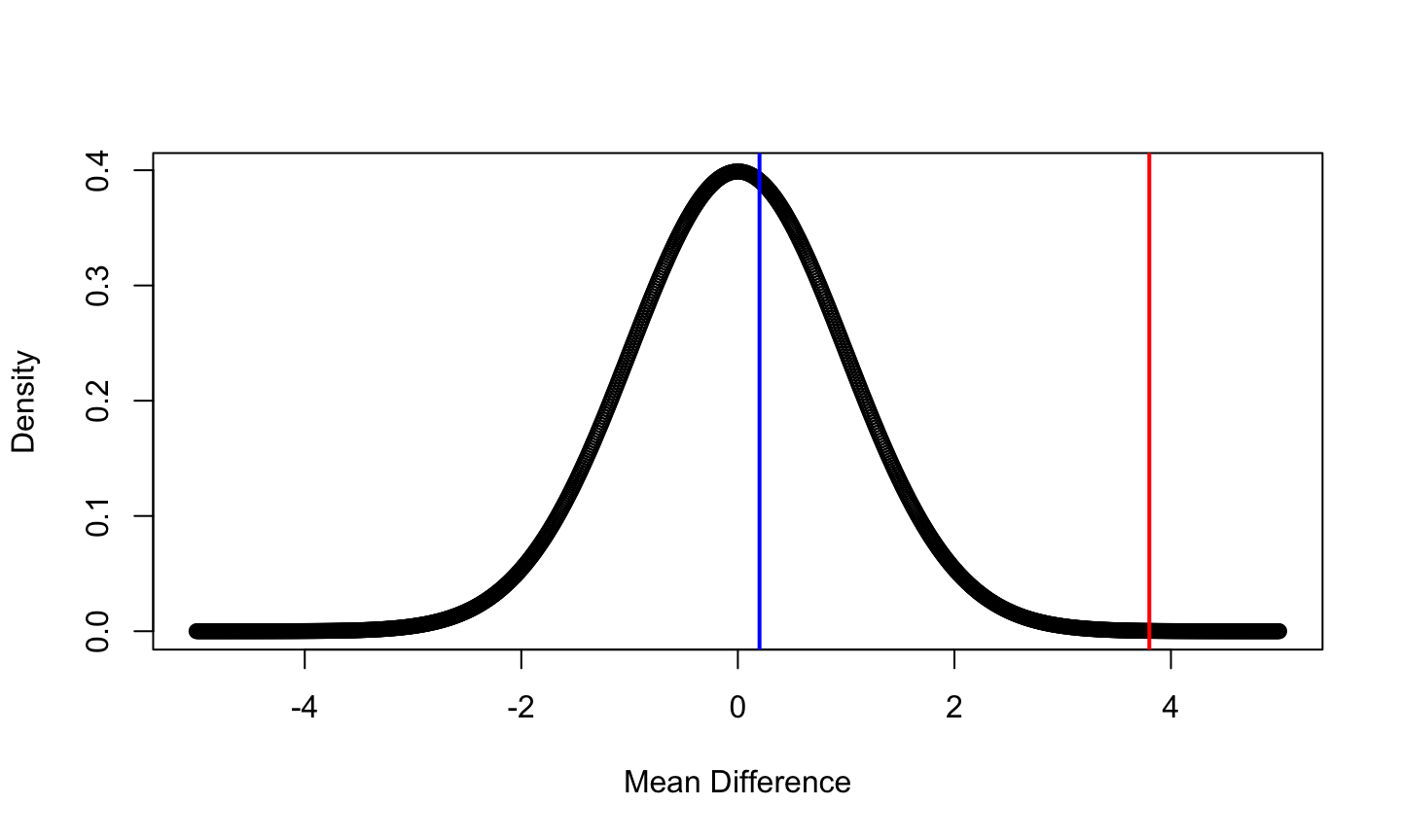
Assume that you want to test whether a drug reduces blood pressure. A sample of size 100 is collected.
- The mean difference between blood pressure before and after taking the medication is 0.2
- The mean difference between blood pressure before and after taking the medication is 3.8
Example
Assume that you want to test whether a drug reduces blood pressure.
- \(H_0\) : The drug does not reduce BP
- \(H_1\) : The drug reduces BP
In notation
- \(H_0\) : \(\Delta = 0\)
- \(H_1\) : \(\Delta > 0\)
where \(\Delta\) is the BP before taking the medicine minus BP after taking the medicine.
Test Types
Two-tailed test
Right-tailed test
Left-tailed test
\(H_0:\ \mu = 8.6,\quad H_1:\ \mu>8.6\) : Right-tailed
\(H_0:\ p =\frac{18}{1000} ,\quad H_1:\ p<\frac{18}{1000}\) : Left-tailed
\(H_0:\ \beta = 0,\quad H_1:\ \beta\neq 0\) : Two-tailed
Procedure
After stating the hypotheses, the researcher designs the study.
Select the correct statistical test
Choose an appropriate level of significance
Formulate a plan for conducting the study
A statistical test uses the data obtained from a sample to make a decision about whether the null hypothesis should be rejected.
The numerical value obtained from a statistical test is called the test value or test statistic.
More on test Statistic
A test statistic is used to decide between \(H_0\) and \(H_a\).
It’s a function of the data (and possibly the parameters in the hypotheses) that measures the support of the data for the \(H_a\).
Assuming \(H_0\) is true (which is why it is called the null or default hypothesis), we determine the sampling distribution (at least approximately) of the test statistic.
We can assess what a typical test statistic would be if \(H_0\) is true, and what would be an unusual test statistic.
The distribution of the test statistic assuming \(H_0\) is true is called the null distribution.
What can happen
- \(H_0\) is true and we do not reject \(H_0\) :
- \(H_0\) is true but we reject \(H_0\):
- \(H_0\) is false and we do not reject \(H_0\) :
- \(H_0\) is false and we reject \(H_0\) :
What can happen
- \(H_0\) is true and we do not reject \(H_0\) : Correct Decision
- \(H_0\) is true but we reject \(H_0\):
- \(H_0\) is false and we do not reject \(H_0\) :
- \(H_0\) is false and we reject \(H_0\) : Correct Decision
What can happen
- \(H_0\) is true and we do not reject \(H_0\) : Correct Decision
- \(H_0\) is true but we reject \(H_0\): Error Type I
- \(H_0\) is false and we do not reject \(H_0\) :
- \(H_0\) is false and we reject \(H_0\) :
What can happen
- \(H_0\) is true and we do not reject \(H_0\) : Correct Decision
- \(H_0\) is true but we reject \(H_0\): Error Type I
- \(H_0\) is false and we do not reject \(H_0\) : Error Type II
- \(H_0\) is false and we reject \(H_0\) : Correct Decision
More Definitions
- Level of Significance - is the maximum probability of committing a Type I error. This probability is symbolized by α. P(type I error) = α
- Critical Value (CV) : separates the critical region from the non-critical region.
- Critical or Rejection Region : is the range of values of the test value that indicates that there is a significant difference and that the null hypothesis should be rejected.
Traditional Method
- State the hypotheses and identify the claim
- Find the critical value using
qnormorqtetc. - Compute the test value
- Make the decision to reject or not reject the null hypothesis
- Summarize the results.
P-value
The P-value (or probability value) is the probability of getting a sample statistic (such as the sample mean) or a more extreme sample statistic in the direction of the alternative hypothesis when the null hypothesis is true.
\[P(\text{Rejecting } H_0|H_0)\]
The P-value is the actual area under the standard normal distribution curve of the test value or a more extreme value (further in the tail).
The smaller the P-value, the stronger the evidence is against \(H_0\).
P-value method
- If p-value is \(\leq \alpha\) then we reject the null hypothesis
- If p-value is \(> \alpha\) then we fail to reject the null hypothesis
Example
Suppose you have a left-tailed test and find the area in the tail to be 0.0489. What is the P-value? Would you reject this at \(\alpha\) = 0.05? \(\alpha\) = 0.01?
Example
Suppose you have a two-tailed test and find the area in one tail to be 0.0084. What is the P-value? Would you reject this at α = 0.05? α = 0.01?
Strength of Evidence
| p-value | Evidence |
|---|---|
| p-value > 0.10 | No evidence for \(H_a\) |
| 0.05 < p-value \(\leq\) 0.10 | Weak evidence for \(H_a\) |
| 0.01 < p-value \(\leq\) 0.05 | Moderate evidence for \(H_a\) |
| 0.001 < p-value \(\leq\) 0.01 | Strong evidence for \(H_a\) |
| p-value \(\leq\) 0.001 | Very strong evidence for \(H_a\) |
Power
Power is the probability of rejecting the null hypothesis when, in fact, it is false.
Power is the probability of making a correct decision (to reject the null hypothesis) when the null hypothesis is false.
Power is the probability that a test of significance will pick up on an effect that is present.
Power is the probability that a test of significance will detect a deviation from the null hypothesis, should such a deviation exist.
Power is the probability of avoiding a Type II error.
\[P(\text{Rejecting }H_0|H_1)\]
Power depends on
- Significance level (or alpha)
- Sample size
- Variability, or variance, in the measured response variable
- Magnitude of the effect of the variable
- Analysis method
Confidence Interval
Review
A confidence interval provides us with plausible values of a target parameter.
A confidence interval has an associated confidence level.
- Under repeated independent trials, a confidence interval procedure will produce intervals containing the target parameter with probability equal to the confidence level.
The formulas for confidence intervals are usually derived from a pivotal quantity.
- A pivotal quantity is a function of the data and the target parameter whose distribution does not depend on the value of the target parameter.
Example
Suppose \(Y_1, Y_2, \dots , Y_n \sim N(\mu, 1)\) and i.i.d.
The random variable \[Z=\frac{\overline{Y}-\mu}{1/\sqrt{n}}\sim N(0,1)\] is a pivotal quantity.
Since \(P(-1.96\leq Z\leq 1.96) = 0.95\), we can derive that \[P\left(\overline{Y} - 1.96 \times \frac{1}{\sqrt{n}} \leq \mu \leq \overline{Y} + 1.96 \times \frac{1}{\sqrt{n}}\right)=0.95 \] Our 95% confidence interval for \(\mu\) (in this context) is \[\left[\overline{Y} - 1.96 \times \frac{1}{\sqrt{n}}, \overline{Y} + 1.96 \times \frac{1}{\sqrt{n}}\right].\]
Example
If \(\overline{y} = 0.551\), then the associated 95% confidence interval for \(\mu\) when \(n=10\) is [-0.070,1.171].
Note: the confidence level is associated with the procedure, not a specific interval.
- A 95% confidence interval procedure will produce intervals that contain the target parameter 95% of the time.
If we used the CI formula given above to produce 100 intervals from independent data sets, then about 95% of them would contain the true mean, but about 5% would not.
Interpretation
CI and Hypothesis Test
CIs are directly linked to hypothesis tests.
A 100(1-\(\alpha\))% two-sided confidence interval for target parameter \(\theta\) is linked with a hypothesis test of \(H_0:\theta=c\) versus \(H_a:\theta\neq c\) tested at level \(\alpha\).
Any point that lies within the \(100(1-\alpha)\)% confidence interval for \(\theta\) represents a value of \(c\) for which the associated null hypothesis would not be rejected at significance level \(\alpha\).
Any point outside of the confidence interval is a value of \(c\) for which the associated null hypothesis would be rejected.
Similar relationships hold for one-sided CIs and hypothesis tests.
Example
Consider the 95% confidence interval for \(\mu\) we previously constructed [-0.070,1.171].
Consider a statistical test of \(H_0:\mu=c\) versus \(H_a:\mu\neq c\) using \(\alpha=0.05\).
For what values of \(c\) would we fail to reject \(H_0\)?
.
.
.
For what values of \(c\) would we reject \(H_0\)?
CI vs Hypothesis Test
A CI provides us with much of the same information as a hypothesis test, but it doesn’t provide the p-value or allow us to do hypothesis tests at different significance levels.
Confidence regions are often preferred over hypothesis tests because they provide additional information in the form of plausible parameters values.
Bootstrap Confidence Intervals
The conventional parametric confidence interval assumes we know the distribution of the population in order to find a pivotal quantity.
- The population distribution is needed to determine the sampling distribution of our statistic.
A bootstrap confidence interval can be constructed if the population distribution is unknown.
Lack of Theory?
How would we estimate the sampling distribution of a statistic without statistical theory?
Estimating the Sampling Distribution of a statistic for a Known Population
- Obtain a random sample of size n from the population.
- Compute the statistic for the random sample.
- Perform steps 1 and 2 a large number of times.
- Determine the empirical distribution of the statistics from the independent samples.
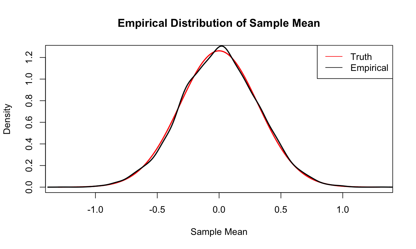
Consider a comparison of the estimated sampling distribution (the empirical distribution) and the true sampling distribution of \(\overline{Y}\) when sampling \(n=10\) observations from a \(N(0,1)\) population.
Sampling Distribution of \(\overline{Y}\)
Let, \(Y_1,\dots, Y_10\sim N(0,1)\), so, \(\overline{Y}\sim N(0, 1/n)\).
Bootstrap Method
The bootstrap method allows us to approximate the sampling distribution of a statistic by using the observed data to produce simulated data sets.
The bootstrap method uses the observed data to approximate the shape, spread, and bias of the sampling distribution of a statistic.
A bootstrap sample is a sample with replacement of size n from the observed data.
Estimation using Bootstrap
Estimating the Sampling Distribution Using the Bootstrap Method
- Obtain a bootstrap sample of the observed data by selecting with replacement a sample of size n from the observed data.
- Compute the statistic for the random sample.
- Perform steps 1 and 2 a large number of times.
- Determine the empirical distribution of the statistics from the independent bootstrap samples (a.k.a., the bootstrap distribution).
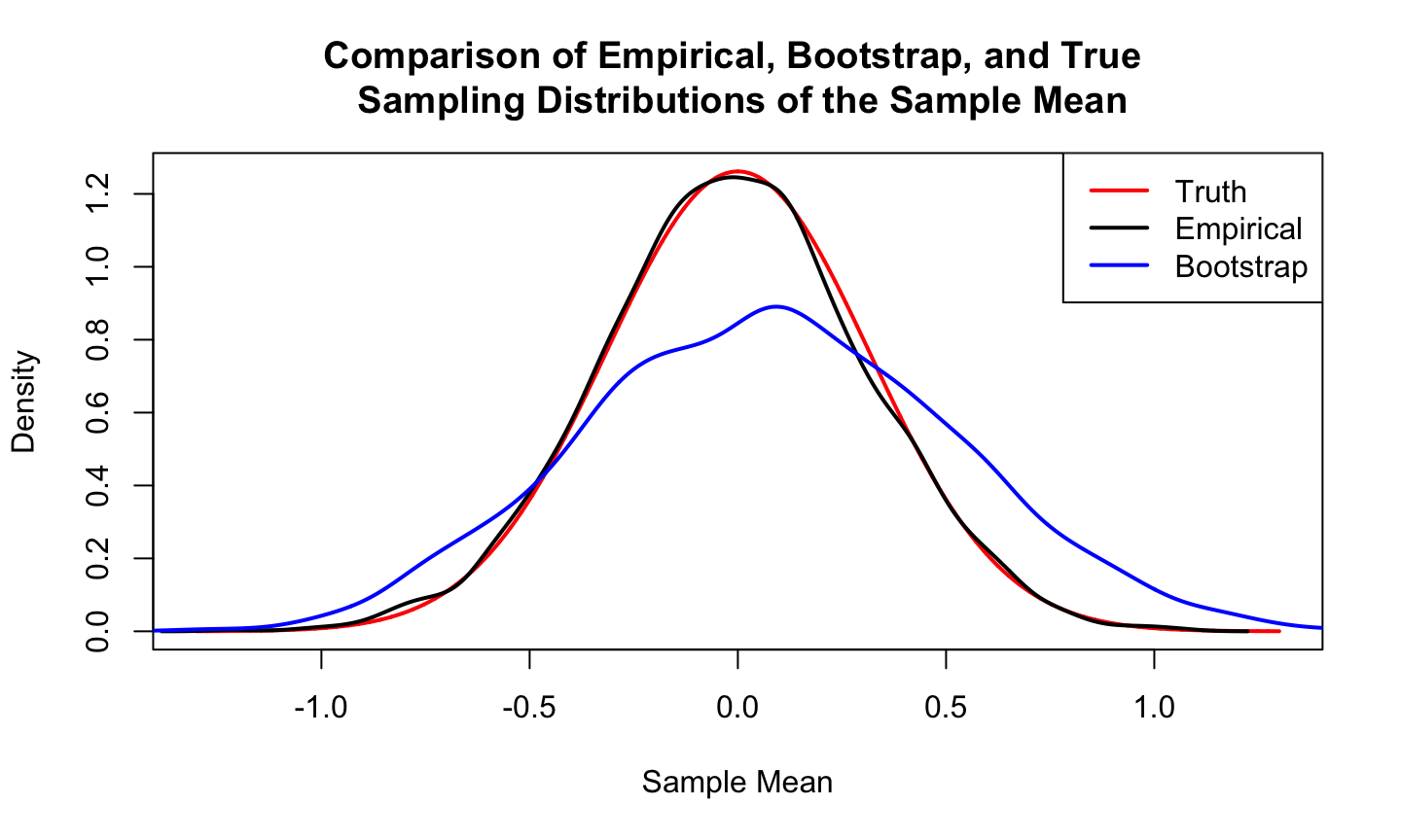
Consider a comparison of the bootstrap, empirical, and true sampling distributions of \(\overline{Y}\) when the data are obtained from a \(N(0,1)\) population.
Comparison
set.seed(10)
x = seq(-1.3, 1.3, length.out = 10000)
Truth = dnorm(x, sd = 1/sqrt(10))

nsim = 4000
Empirical = sapply(1:nsim, function(x) mean(rnorm(10)))

y = rnorm(10)
boot_ybar = sapply(1:nsim, function(x) mean(sample(y, replace = T)))

plot(x,Truth,col='red',type = 'l', lwd = 2,
     xlab = 'Sample Mean', ylab = 'Density',
     main = 'Comparison of Empirical, Bootstrap, and True \n Sampling Distributions of the Sample Mean')
lines(density(Empirical), lwd = 2)
lines(density(boot_ybar),lwd = 2, col='blue')
legend('topright',legend = c('Truth','Empirical','Bootstrap'),
       col = c('red','black','blue'), lty = 1,lwd = 2)
Comparison
CI from Bootstrap
A 100(1-\(\alpha\))% confidence interval for a target parameter \(\theta\) can be obtained by determining the \(\alpha\)/2 and 1-\(\alpha\)/2 quantiles of the bootstrap distribution for \(\hat{\theta}\). E.g., a 95% CI for a population mean \(\mu\) could be obtained by taking the 0.025 and 0.975 quantiles of the bootstrap distribution for \(\overline{Y}\).
Example (continued): Continuing our previous example, the 95% bootstrap confidence interval for \(\mu\) is.
quantile(boot_ybar, prob = c(0.025, 0.975))
##       2.5%      97.5%
## -0.7689507  0.9525203
The parametric 95% confidence interval is [-0.070,1.171].
Suggestion
The parametric and bootstrap methods of constructing confidence intervals will NOT produce identical intervals, though the intervals should be similar if the distributional assumptions are satisfied.
If you are unsure whether the distributional assumptions are satisfied, you should use the bootstrap method to construct your confidence interval.
Exercise
Grogan and Wirth (1981) provide data on the wing length in millimeters of nine members of a species of midge (small, two-winged flies). From these nine measurements, we wish to make inference about the population mean \(\mu\). Assume that the data are an i.i.d. sample from a \(N(\mu,\sigma^2)\) population with \(\mu\) and \(\sigma^2\) unknown.
The data are: 1.64, 1.70, 1.72, 1.74, 1.82, 1.82, 1.82, 1.90, 2.08
- Construct a 98% parametric confidence interval for \(\mu\).
- Construct a 98% bootstrap confidence interval for \(\mu\).
- Perform a hypothesis test of whether \(\mu\)>2 at \(\alpha\)=0.02.
Solution
dat = c(1.64, 1.70, 1.72, 1.74, 1.82, 1.82, 1.82, 1.90, 2.08)
ybar = mean(dat)
s = sd(dat)
er = qt(0.99, df = length(dat)-1) * s/sqrt(length(dat))
print(paste0('98% parametric CI is [', round(ybar - er,3), ', ', round(ybar +er,3),']'))
## [1] "98% parametric CI is [1.679, 1.93]"
boot_ybar = sapply(1:4000, function(x) mean(sample(dat, replace = T)))
print(paste0('98% bootstrap CI is [',round(quantile(boot_ybar, probs = 0.025),3),', ',
             round(quantile(boot_ybar, probs = 0.975),3),']'))
## [1] "98% bootstrap CI is [1.731, 1.887]"
ttest = (ybar - 2)/(s/sqrt(length(dat)))
print(paste0('t-test statistics: ', round(ttest,3)))
## [1] "t-test statistics: -4.516"
print(paste0('p-value:', round(1-pt(ttest,df = length(dat)-1) ,3)))
## [1] "p-value:0.999"