Given a new set of regressor values, \(x_0=(1,x_{01},…,x_{0,p-1} )^T\), a natural predictor for the associated response is \(\hat{y}_0 = x_0^T\hat{\beta}\).

What is the uncertainty in our prediction?

• It depends on the type of prediction made.

There are two types of predictions that are made from regression models.

1. Prediction of the mean response.
2. Prediction of a future (or new) observation

Consider building a regression model predicting the selling price of homes in a certain area based on predictors such as the number of bedrooms and closeness to a major highway.

Consider building a regression model predicting the selling price of homes in a certain area based on predictors such as the number of bedrooms and closeness to a major highway.

Given a set of regressor values x_0, we might want to:

• Estimate the average selling price of a house with characteristics \(x_0\).
  • The average selling price is \(x_0^T \beta\), and we would estimate the average price by \(\hat{y}_0=x_0^T \hat{\beta}\).
    
  • The parametric uncertainty of our estimate is only affected by our uncertainty in estimating \(\beta\).
  • Called prediction or estimation of the mean response

• Predict the future selling price of a specific house with characteristics \(x_0\).

  • The selling price of this house is \(y_0=x_0^T \beta+\epsilon_0\).
    
  • Since \(E(\epsilon_0 |X=x_0 )=0\), the predicted price for a new observation is also \(\hat{y}_0+\hat{\epsilon}_0=x_0^T \hat{\beta}+0=x_0^T \hat{\beta}\)
    
  • The parametric uncertainty of our prediction is affected by our uncertainty in estimating \(\beta\) and the uncertainty associated with the error \(\epsilon_0\).
  • Called Prediction of a new or future response

\[\begin{aligned} var(x_0^T\hat{\beta}) = & var(x_0^T(X^TX)^{-1}X^Ty) \\ = & x_0^T(X^TX)^{-1}X^T var(y) \left(x_0^T(X^TX)^{-1}X^T\right)^T\\ =& x_0^T(X^TX)^{-1}X^T var(y) X(X^TX)^{-1}x_0\\ =& x_0^T(X^TX)^{-1}X^T \sigma^2 I X(X^TX)^{-1}x_0\\ =& x_0^T(X^TX)^{-1}X^T X(X^TX)^{-1}x_0 \sigma^2\\ =& x_0^T(X^TX)^{-1}x_0 \sigma^2\\ \end{aligned}\]

\[\begin{aligned} var(x_0^T\hat{\beta} +\epsilon) = & var(x_0^T(X^TX)^{-1}X^Ty) +\sigma^2 & \text{Assume Independence}\\ =& \left(1+x_0^T(X^TX)^{-1}x_0\right) \sigma^2 \\ \end{aligned}\]

Since, \(\hat{y}_0 = x_0^T\hat{\beta} \sim N(x_0^T\beta, x_0^T(X^TX)^{-1}x_0 \sigma^2\),

\[\frac{\hat{y}_0 - x_0^T\beta}{\hat{\sigma}\sqrt{x_0^T(X^TX)^{-1}x_0}}\sim T_{n-p}.\]

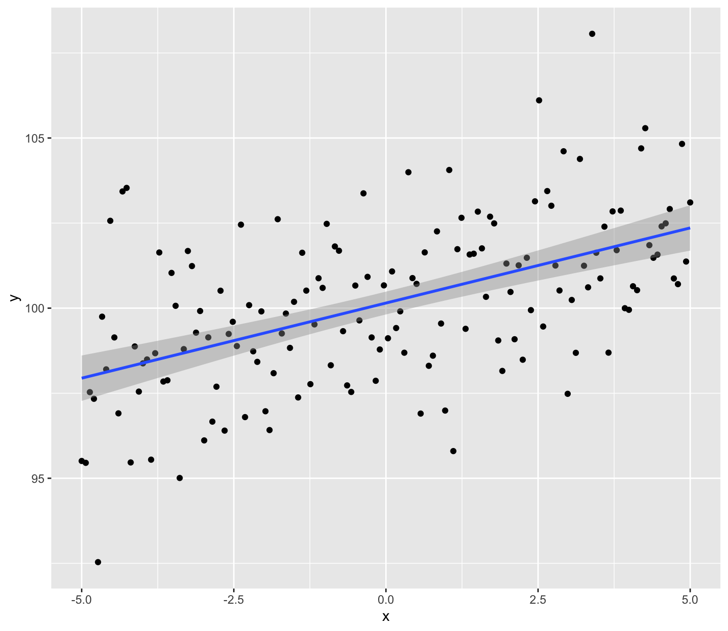
A 100(1-)% CI for the mean response given \(x_0\), \[x_0^T\hat{\beta} \pm t_{n-p}^{\alpha/2} \hat{\sigma}\sqrt{x_0^T(X^TX)^{-1}x_0}.\]

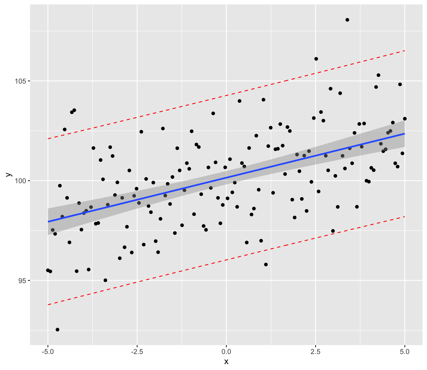
A 100(1-)% CI for a future response given \(x_0\), \[x_0^T\hat{\beta} \pm t_{n-p}^{\alpha/2} \hat{\sigma}\sqrt{1+x_0^T(X^TX)^{-1}x_0}.\]

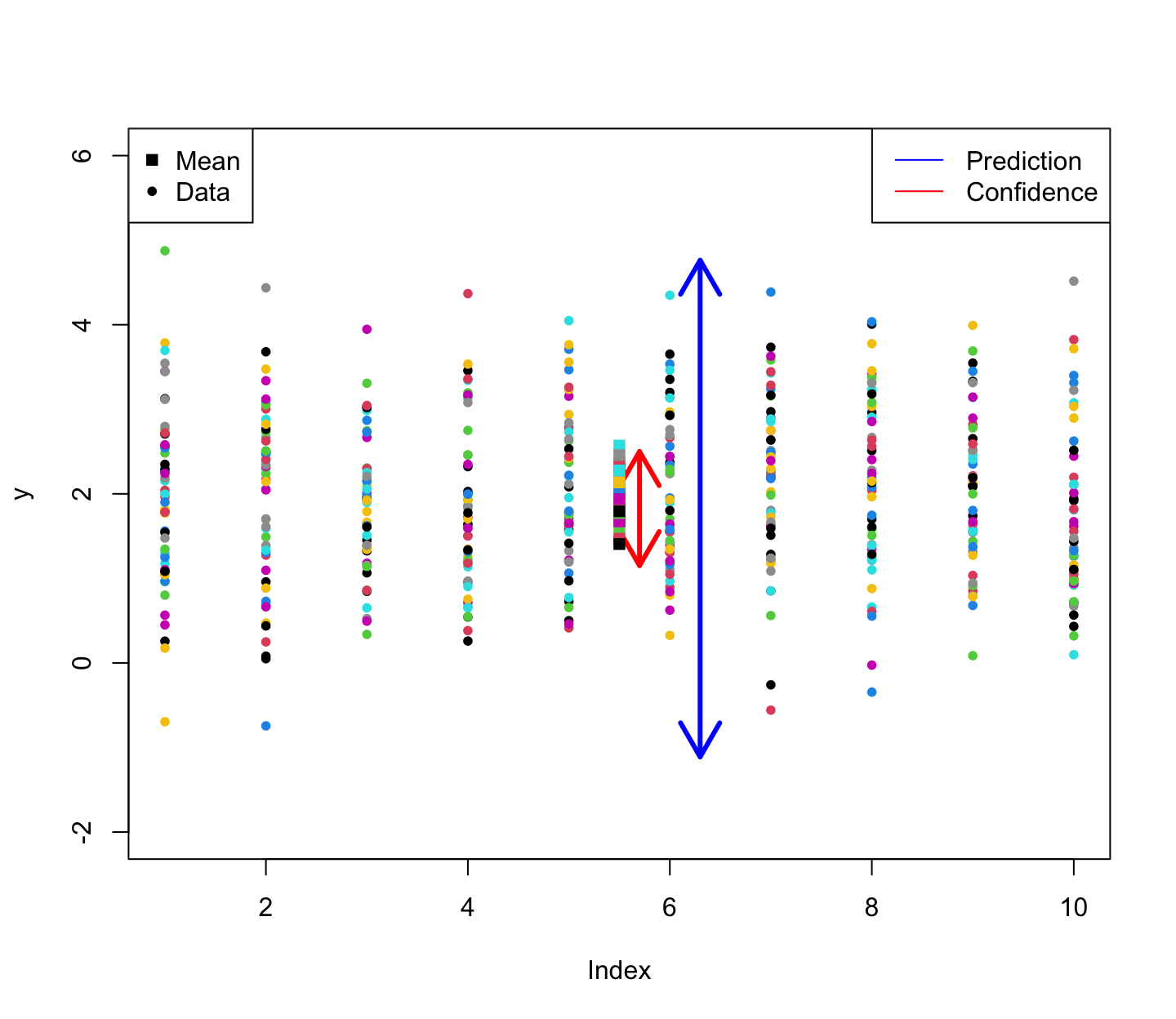
A future observation is a random variable. Thus, the second type of interval is typically called a prediction interval (PI).

• There is a 95% chance that the actual future value will fall within our prediction interval (in the context of constructing many intervals from independent samples of the population and our assumptions are correct).

A confidence interval for the mean response is typically much narrower than the prediction interval for a new response (assuming the same x_0).

arrows(x0 = 5.7, y0 = ci(y)[1], x1 = 5.7, y1 = ci(y)[2], lwd = 3, code = 3, col = 'red')

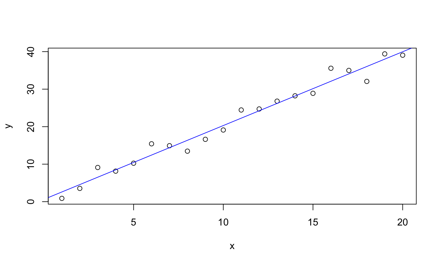
set.seed(123)
x = seq(1,20)
y = 2*x + rnorm(length(x), mean = 0, sd = 2)
lmod = lm(y~x)
plot(x,y)
abline(lmod, col = 'blue')

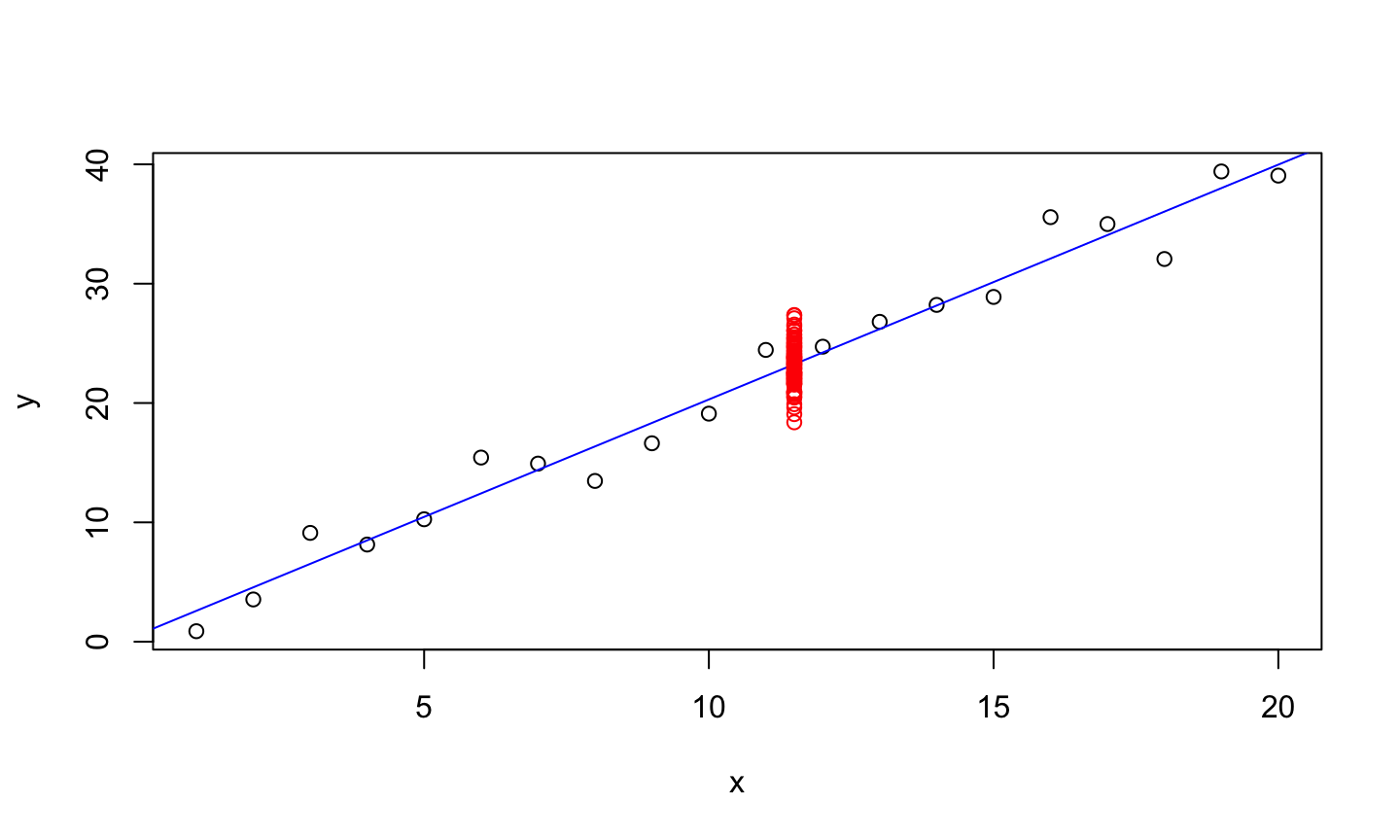
set.seed(123)
new_obs = 2*11.5 + rnorm(100, mean = 0, sd = 2)
plot(x,y)
abline(lmod, col = 'blue')
points(rep(11.5, length(new_obs)), new_obs, col='red')

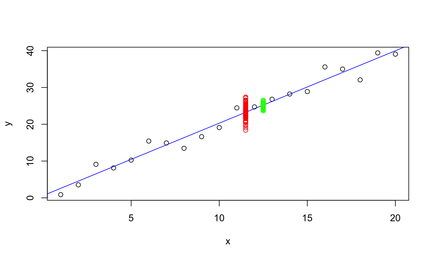
set.seed(123)
mean_obs <- c()
for(i in 1:100){
  obs = 2*12.5 + rnorm(10, mean = 0, sd = 2)
  mean_obs[i]<-mean(obs)
}
plot(x,y)
abline(lmod, col = 'blue')
points(rep(11.5, length(new_obs)), new_obs, col='red')
points(rep(12.5, length(mean_obs)), mean_obs, col = 'green')

Measuring body fat is not simple. Muscle and bone are denser than fat so an estimate of body density can be used to estimate the proportion of fat in the body. Measuring someone’s weight is easy but volume is more difficult. One method requires submerging the body underwater in a tank and measuring the increase in the water level. Most people would prefer not to be submerged underwater to get a measure of body fat, so we would like an easier method. In order to develop such a method, researchers recorded age, weight, height, and 10 body circumference measurements for 252 men. Each man’s percentage of body fat was accurately estimated by an underwater weighing technique. Can we predict body fat using only the easy-to-record measurements?

x <- model.matrix(lmod)
(x0<-apply(x, 2, median))

## (Intercept)         age      weight      height        neck       chest 
##        1.00       43.00      176.50       70.00       38.00       99.65 
##       abdom         hip       thigh        knee       ankle      biceps 
##       90.95       99.30       59.00       38.50       22.80       32.05 
##     forearm       wrist 
##       28.70       18.30

(y0<-sum(x0*coef(lmod)))

## [1] 17.49322

predict(lmod, newdata = data.frame(t(x0)))

##        1 
## 17.49322

Note: The data.frame object placed in the new argument must include columns with names matching the names of the predictor variables in the fitted model.

predict(lmod, newdata = data.frame(t(x0)), interval = "prediction", level = 0.95)

##        fit     lwr      upr
## 1 17.49322 9.61783 25.36861

predict(lmod, newdata = data.frame(t(x0)), interval = "confidence", level = 0.95)

##        fit      lwr      upr
## 1 17.49322 16.94426 18.04219

The prediction interval ranges from 9.6% body fat up to 25.4%. This is pretty wide, so there may not be enough information for practical use.

The confidence interval for the mean response is 16.9% to 18.1%, which is much narrower.

The percentage of body fat between 16.94 and 18.04 are good estimates of the unknown mean percent body fat of the people with age –, height –, etc. In general, if we would repeat our sampling procedure infinitely, 95% of such constracted confidence intervals would contain the true mean percentage of body fat.

Given a person’s measurements are (age = 43, height = 70, etc.), the percengate of body fat will be between 9.62 to 25.37 with a confidence of 95%. In general, if we could repeat our sampling process infinitely, 95% of such constructed prediction intervals would contain the person’s true percent body fat.

Extrapolation is making statistical inference outside the range of the observed data.

• Quantitative extrapolation concerns x_0 that are far from the original data.
• Prediction intervals become wider as we move away from the observed data.

What happens when we predict body fat at the 95th percentile of the observed data?

(x1 <- apply(x,2,function(x) quantile(x,0.95)))

## (Intercept)         age      weight      height        neck       chest 
##       1.000      67.000     225.650      74.500      41.845     116.340 
##       abdom         hip       thigh        knee       ankle      biceps 
##     110.760     112.125      68.545      42.645      25.445      37.200 
##     forearm       wrist 
##      31.745      19.800

predict(lmod, new = data.frame(t(x1)), interval="prediction")

##        fit      lwr      upr
## 1 30.01804 21.92407 38.11202

predict(lmod, new = data.frame(t(x1)), interval="confidence")

##        fit      lwr      upr
## 1 30.01804 28.07072 31.96537

Our confidence interval for the mean is almost 4% wide instead of 1%! That is a large increase in our uncertainty!

An additional source of variation is not accounted for in the previous intervals:

• What is the correct model for this data?

We do our best to find a good model given the available data, but there will always be substantial model uncertainty, i.e., the form the model should take.

Parametric uncertainty is accounted for using the methods we have learned.

Model uncertainty is much harder to quantify.

• Bad model. The statistician does a poor job of modeling the data.

• Quantitative extrapolation. We try to predict outcomes for cases with predictor values much different from what we see in the data.

  • This is a practical problem in assessing the risk from low exposure to substances that are dangerous in high quantities — consider second-hand tobacco smoke, asbestos, and radon.

• Qualitative extrapolation. We try to predict outcomes for observations that come from a different population.

  • We used the body fat model for men to predict the body fat for women.
  • This is a common problem because circumstances are always changing and it’s hard to judge whether the new case is comparable.
  • We prefer experimental data to observational data, but sometimes experience from the laboratory does not transfer to real life.

• Overconfidence due to overtraining.

  • Data analysts search for a model that fits their observed data very closely, but the fitted model may not be appropriate for new data.
  • This can lead to unrealistically small σ ̂.

• Black swans. Sometimes errors can appear to be normally distributed because you haven’t seen enough data to be aware of extremes.

  • This is of particular concern in financial applications where stock prices are characterized by mostly small changes (normally distributed) but with infrequent large changes (usually falls).