6/3/2020
Variable Selection
Summary
- Forward- and backward-stepwise selection
- Different selection criteria:
- Adjusted \(R^2\)
- AIC
- BIC
- Mallow’s \(C_p\)
- Training and Test error on prediction
- Cross-validation
What missed
set.seed(105)
x<-runif(100)
y<-x + rnorm(100, mean = 0, sd = 0.05)
z<- 1+2*x - 3*y + rnorm(100,mean = 0, sd = 1)
plot3d(x,y,z)
cor(x,y)
## [1] 0.9871729
You must enable Javascript to view this page properly.
Individual predictors
summary(lm(z~x))
##
## Call:
## lm(formula = z ~ x)
##
## Residuals:
##      Min       1Q   Median       3Q      Max
## -2.26590 -0.64277  0.06263  0.66831  2.00946
##
## Coefficients:
##             Estimate Std. Error t value Pr(>|t|)
## (Intercept)   0.8577     0.1913   4.483    2e-05 ***
## x            -0.6260     0.3341  -1.874    0.064 .
## ---
## Signif. codes:  0 '***' 0.001 '**' 0.01 '*' 0.05 '.' 0.1 ' ' 1
##
## Residual standard error: 0.9116 on 98 degrees of freedom
## Multiple R-squared:  0.03458,    Adjusted R-squared:  0.02473
## F-statistic:  3.51 on 1 and 98 DF,  p-value: 0.06397
Individual predictors
summary(lm(z~I(x+y)))
##
## Call:
## lm(formula = z ~ I(x + y))
##
## Residuals:
##      Min       1Q   Median       3Q      Max
## -2.24803 -0.64922  0.07512  0.66991  2.02239
##
## Coefficients:
##             Estimate Std. Error t value Pr(>|t|)
## (Intercept)   0.8759     0.1902   4.605 1.24e-05 ***
## I(x + y)     -0.3292     0.1650  -1.995   0.0488 *
## ---
## Signif. codes:  0 '***' 0.001 '**' 0.01 '*' 0.05 '.' 0.1 ' ' 1
##
## Residual standard error: 0.9095 on 98 degrees of freedom
## Multiple R-squared:  0.03904,    Adjusted R-squared:  0.02924
## F-statistic: 3.982 on 1 and 98 DF,  p-value: 0.04878
Principal Component
Principal Component in 2D
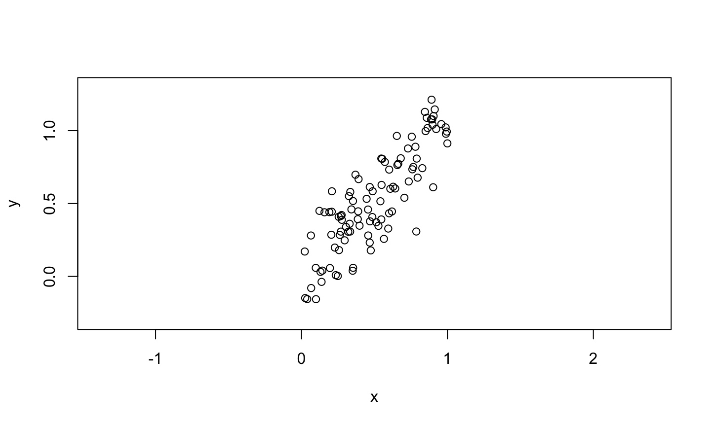
set.seed(105)
x<-runif(100)
y<-x + rnorm(100, mean = 0, sd = 0.2)
plot(x,y, xlim = c(-0.3, 1.3), ylim = c(-0.3, 1.3), asp = 1)
Principal Component in 2D
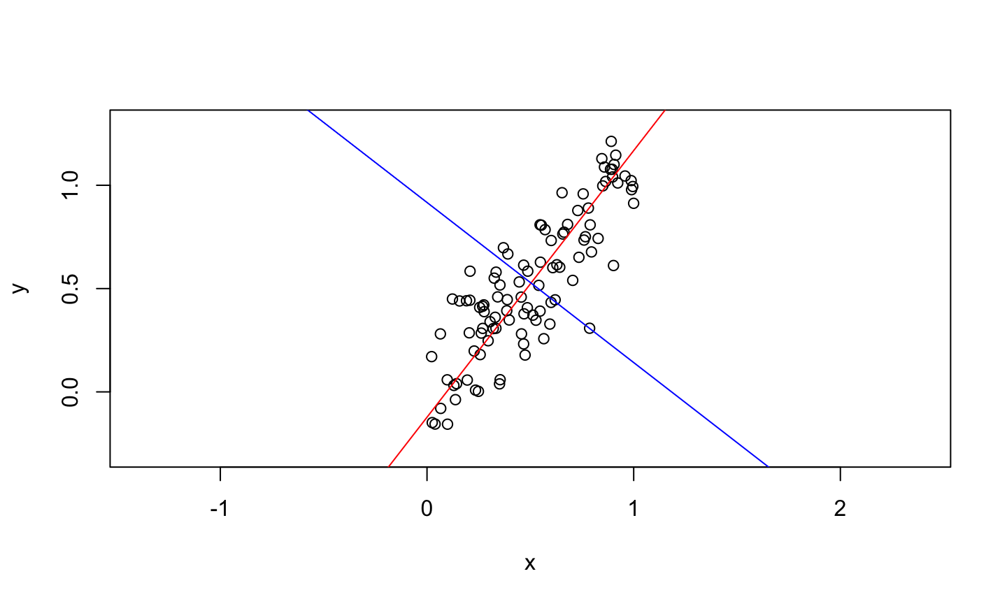
set.seed(105)
x<-runif(100)
y<-x + rnorm(100, mean = 0, sd = 0.2)
plot(x,y, xlim = c(-0.3, 1.3), ylim = c(-0.3, 1.3), asp = 1)
pcs = prcomp(data.frame(x=x,y=y))
slope = pcs$rotation[2,]/pcs$rotation[1,]
abline(coef = c(pcs$center[2] - slope[1]*pcs$center[1], slope[1]), col = 'red')
abline(coef = c(pcs$center[2] - slope[2]*pcs$center[1], slope[2]), col = 'blue')
Principal Component in R
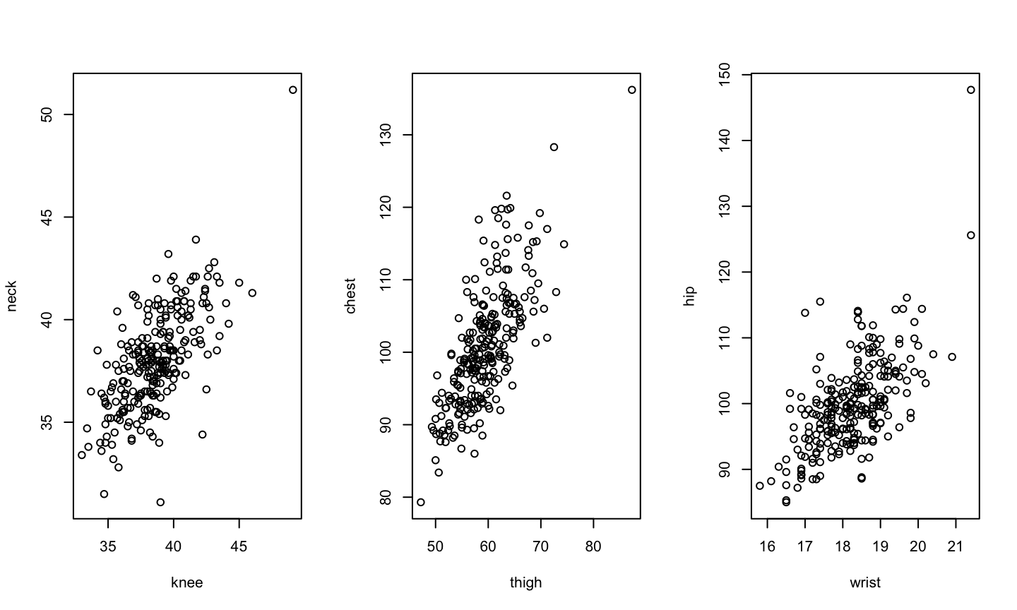
Consider the dimensions of the human body as measured in a study on 252 men as described in Johnson (1996)
data(fat,package="faraway")
par(mfrow = c(1,3))
plot(neck ~ knee, fat)
plot(chest ~ thigh, fat)
plot(hip ~ wrist, fat)
Principal Componenet in R
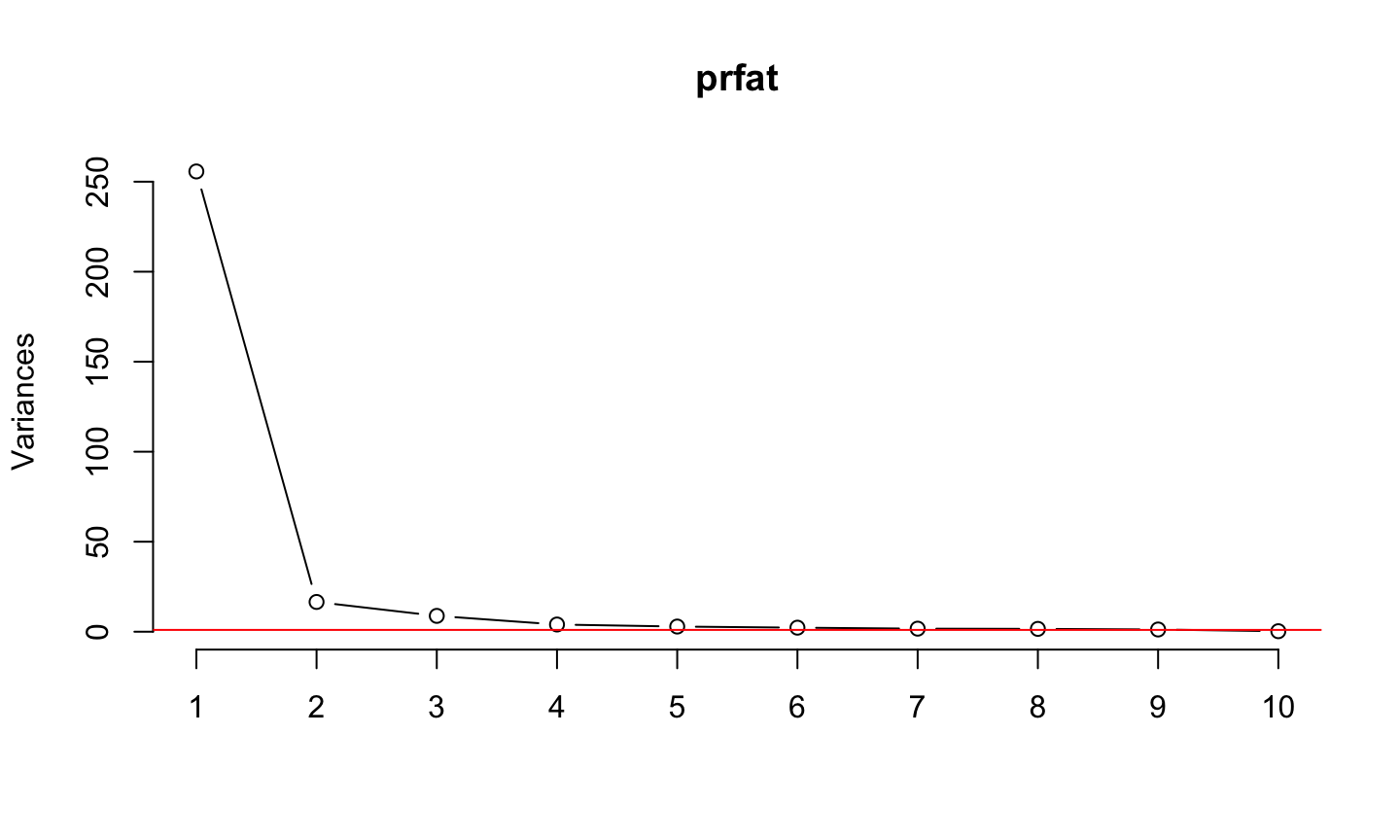
cfat <- fat[,9:18]
prfat <- prcomp(cfat)
dim(prfat$rot)
## [1] 10 10
dim(prfat$x)
## [1] 252 10
summary(prfat)
## Importance of components:
##                           PC1     PC2     PC3     PC4     PC5     PC6     PC7
## Standard deviation     15.990 4.06584 2.96596 2.00044 1.69408 1.49881 1.30322
## Proportion of Variance  0.867 0.05605 0.02983 0.01357 0.00973 0.00762 0.00576
## Cumulative Proportion   0.867 0.92304 0.95287 0.96644 0.97617 0.98378 0.98954
##                            PC8     PC9    PC10
## Standard deviation     1.25478 1.10955 0.52737
## Proportion of Variance 0.00534 0.00417 0.00094
## Cumulative Proportion  0.99488 0.99906 1.00000
Rotation Matrix
round(prfat$rotation[,1:3],2)
##          PC1   PC2   PC3
## neck    0.12 -0.02  0.20
## chest   0.50  0.38  0.64
## abdom   0.66  0.38 -0.55
## hip     0.42 -0.51 -0.18
## thigh   0.28 -0.60  0.02
## knee    0.12 -0.17  0.04
## ankle   0.06 -0.12  0.10
## biceps  0.15 -0.18  0.34
## forearm 0.07 -0.09  0.29
## wrist   0.04 -0.01  0.08
Principal component in R (Scaling)
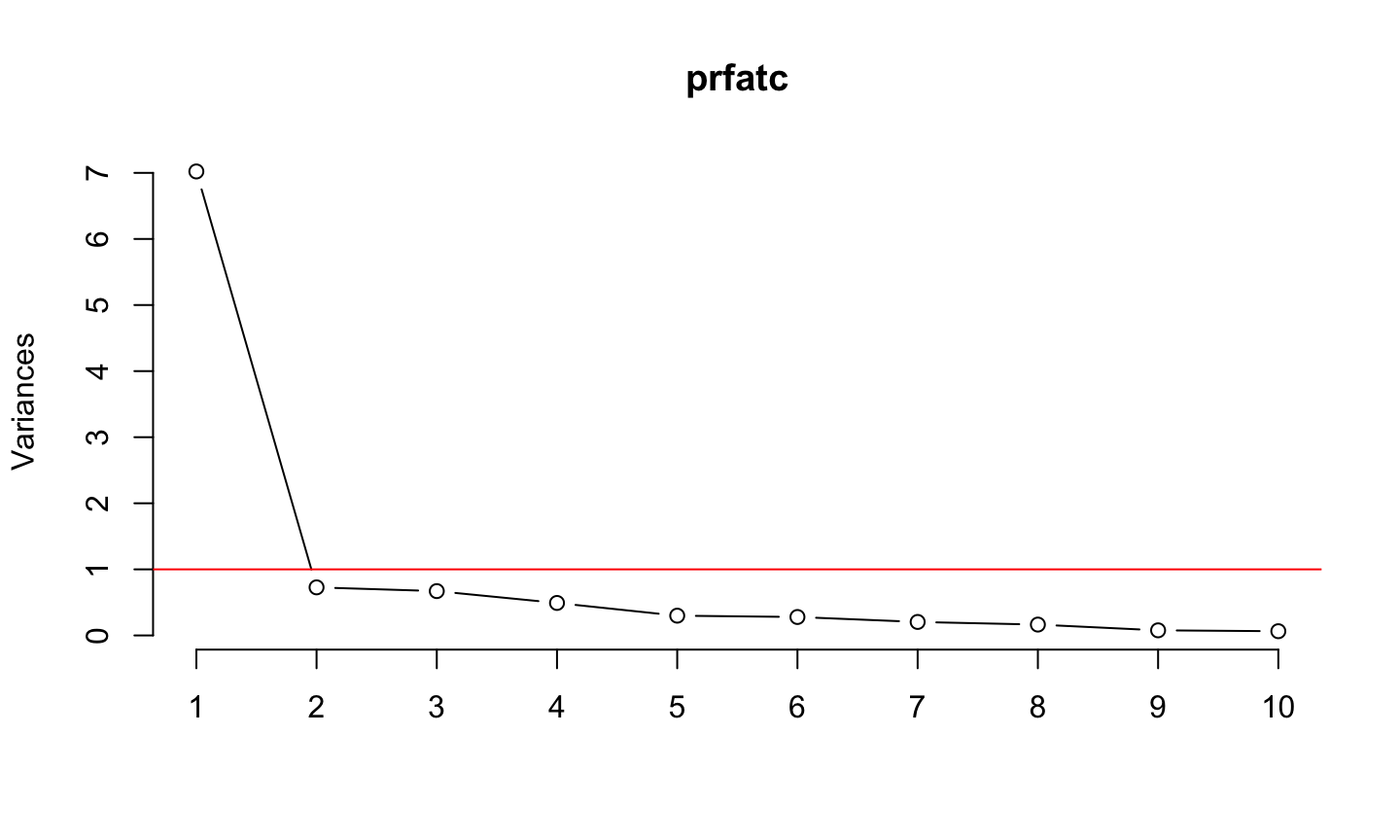
prfatc <- prcomp(cfat, scale=TRUE)
summary(prfatc)
## Importance of components:
##                           PC1     PC2     PC3     PC4     PC5     PC6     PC7
## Standard deviation     2.6498 0.85301 0.81909 0.70114 0.54708 0.52831 0.45196
## Proportion of Variance 0.7021 0.07276 0.06709 0.04916 0.02993 0.02791 0.02043
## Cumulative Proportion  0.7021 0.77490 0.84199 0.89115 0.92108 0.94899 0.96942
##                            PC8     PC9   PC10
## Standard deviation     0.40539 0.27827 0.2530
## Proportion of Variance 0.01643 0.00774 0.0064
## Cumulative Proportion  0.98586 0.99360 1.0000
round(prfatc$rot[,1],2)
##    neck   chest   abdom     hip   thigh    knee   ankle  biceps forearm   wrist
##    0.33    0.34    0.33    0.35    0.33    0.33    0.25    0.32    0.27    0.30
Principal Component in Math
- \(X\) be \(n\times p\) matrix of data points
- We seek for linear combination \(\sum_{j=1}^p a_jx_j = Xa\) so that \(Xa\) has maximum variance
- \(var(Xa) = a^TSa\), where \(S\) is the sample covariance matrix
- We seek for \(a\) that maximizes \(a^TSa\).
- Need \(a^Ta=1\) condition for identifiability
- Lagrange multiplier: \(a^TSa - \lambda(a^Ta-1)\)
- Setting first derivative equals zero \(\Rightarrow\) \(Sa=\lambda a\)
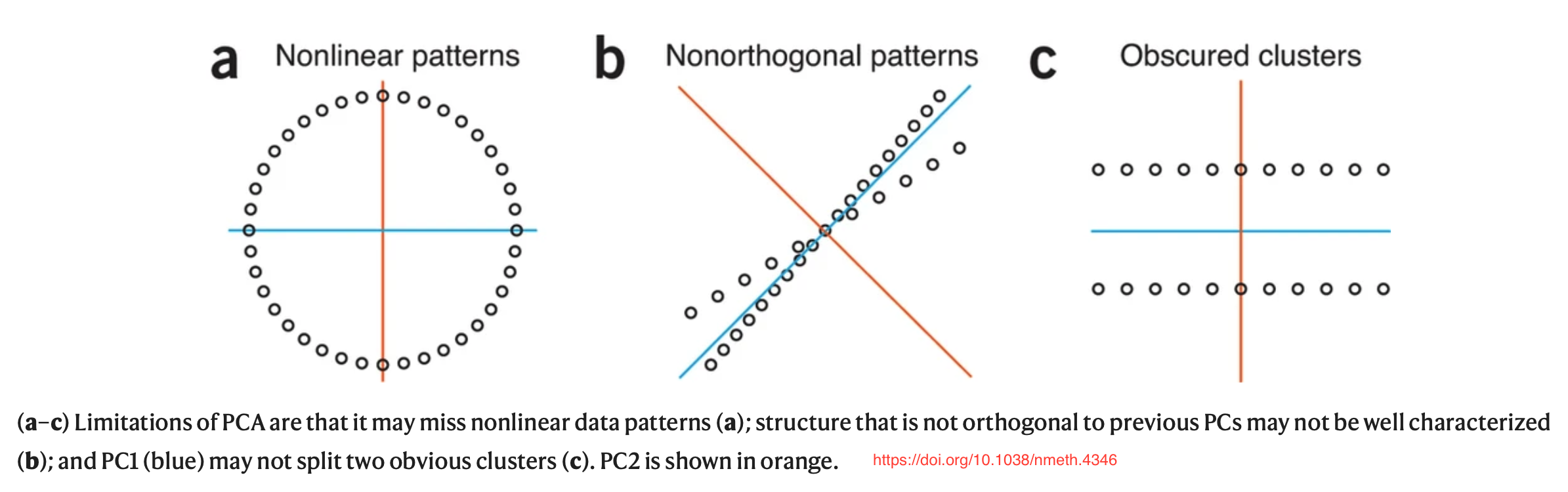
Some limitations
- Sensitive to outliers
- Mahalanobis distance
- \(\sqrt{(x-\mu)^T\Sigma^{-1}(x-\mu)}\)
- \(\sqrt{(x-\mu)^T\Sigma^{-1}(x-\mu)}\)
- Mahalanobis distance
Many different applications
Principal Component Regression
Body measure example
Response: percentage of body fat
lmoda <- lm(fat$brozek ~ ., data=cfat)
sumary(lmoda)
##               Estimate Std. Error t value  Pr(>|t|)
## (Intercept)  7.2287487  6.2143092  1.1632 0.2458816
## neck        -0.5819470  0.2085800 -2.7900 0.0056916
## chest       -0.0908468  0.0854300 -1.0634 0.2886622
## abdom        0.9602291  0.0715821 13.4144 < 2.2e-16
## hip         -0.3913546  0.1126862 -3.4730 0.0006101
## thigh        0.1337081  0.1249222  1.0703 0.2855412
## knee        -0.0940552  0.2123939 -0.4428 0.6582831
## ankle        0.0042223  0.2031754  0.0208 0.9834370
## biceps       0.1111963  0.1591179  0.6988 0.4853321
## forearm      0.3445364  0.1855113  1.8572 0.0644989
## wrist       -1.3534719  0.4714098 -2.8711 0.0044542
##
## n = 252, p = 11, Residual SE = 4.07132, R-Squared = 0.74
Body measure example
lmodpcr <- lm(fat$brozek ~ prfatc$x[,1:2])
sumary(lmodpcr)
##                    Estimate Std. Error t value  Pr(>|t|)
## (Intercept)        18.93849    0.32913 57.5416 < 2.2e-16
## prfatc$x[, 1:2]PC1  1.84198    0.12446 14.8003 < 2.2e-16
## prfatc$x[, 1:2]PC2 -3.55053    0.38661 -9.1837 < 2.2e-16
##
## n = 252, p = 3, Residual SE = 5.22473, R-Squared = 0.55
Body measure example
round(prfatc$rotation[,1:2],2)
##          PC1   PC2
## neck    0.33  0.00
## chest   0.34 -0.27
## abdom   0.33 -0.40
## hip     0.35 -0.25
## thigh   0.33 -0.19
## knee    0.33  0.02
## ankle   0.25  0.62
## biceps  0.32  0.02
## forearm 0.27  0.36
## wrist   0.30  0.38
PC1: overall size PC2: center measures
Scree plot
screeplot(prfatc, type = 'line')
abline(h=1, col='red')
Scree plot
screeplot(prfat, type = 'line')
abline(h=1, col ='red')
Regularization
Penalizing \(\beta\)
x = seq(1,10,length.out = 100)
y = 2+2*x + rnorm(100,0,0.5)
sumary(lm(y~x))
##             Estimate Std. Error t value  Pr(>|t|)
## (Intercept) 2.009651   0.105407  19.066 < 2.2e-16
## x           2.004022   0.017297 115.860 < 2.2e-16
##
## n = 100, p = 2, Residual SE = 0.45390, R-Squared = 0.99
Penalizing \(\beta\)
x1 = x +runif(100,0,0.1)
sumary(lm(y ~ x + x1))
##             Estimate Std. Error t value Pr(>|t|)
## (Intercept)  2.01627    0.12825 15.7215   <2e-16
## x            2.13985    1.48334  1.4426   0.1524
## x1          -0.13582    1.48320 -0.0916   0.9272
##
## n = 100, p = 3, Residual SE = 0.45622, R-Squared = 0.99
Penalizing \(\beta\)
x2 = x + x1 +runif(100,0,0.01)
sumary(lm(y ~ x + x1+x2))
##              Estimate Std. Error t value Pr(>|t|)
## (Intercept)   2.09906    0.14991 14.0024   <2e-16
## x            19.34726   16.22961  1.1921   0.2362
## x1           17.07016   16.22827  1.0519   0.2955
## x2          -17.20637   16.16080 -1.0647   0.2897
##
## n = 100, p = 4, Residual SE = 0.45590, R-Squared = 0.99
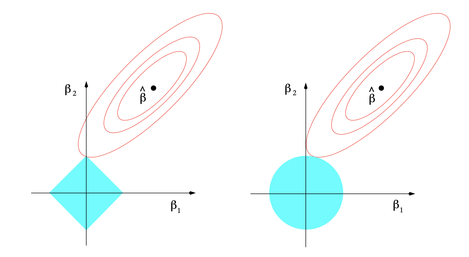
Ridge Regression
Minimize
\[(y-X\beta)^T(y-X\beta) + \lambda \sum\limits_j\beta_j^2\] * \(\lambda\geq 0\) : complexity parameter
- The larger the \(\lambda\), the grater the amount of shrinkage
RSS
\[(y-X\beta)^T(y-X\beta) + \lambda \beta^T\beta\]
Estimate \[\hat{\beta}_\text{ridge} = (X^TX +\lambda I)^{-1}X^Ty\]
Properties
\[\hat{\beta}_\text{ridge} = (X^TX +\lambda I)^{-1}X^Ty\] * Even if \(X^X\) is not of full rank, \(X^TX+\lambda I\) is non-singular
- If predictors are orthonormal \(\hat{\beta}_\text{ridge} = \hat{\beta}/(1-\lambda)\)
Properties
Fitted values Let, \(X=UDV^T\)
OLS \[X\hat{\beta} = X(X^TX)^{-1}X^Ty = UU^Ty\]
Ridge
\[X(X^TX+\lambda I)^{-1}X^Ty = \sum\limits_{j=1}^p u_j \frac{d_j^2}{d_j^2+\lambda} u_j^Ty\]
- Since \(\lambda\geq 0,\) \(\frac{d_j^2}{d_j^2+\lambda}\leq 1\)
- A grater amount of shrinkage is applied to the coordinates of basis vectors with smaller \(d_j^2\)
- \(d_j^2\) are the eigenvalues of \(X^TX\)
Lasso Rigression
L1 Penalty
\[(y-X\beta)^T(y-X\beta) + \lambda \sum\limits_j |\beta_j|\] * No closed form solution
Compare
include_graphics('images/ridge_lasso.png')
Penalized Regression in R
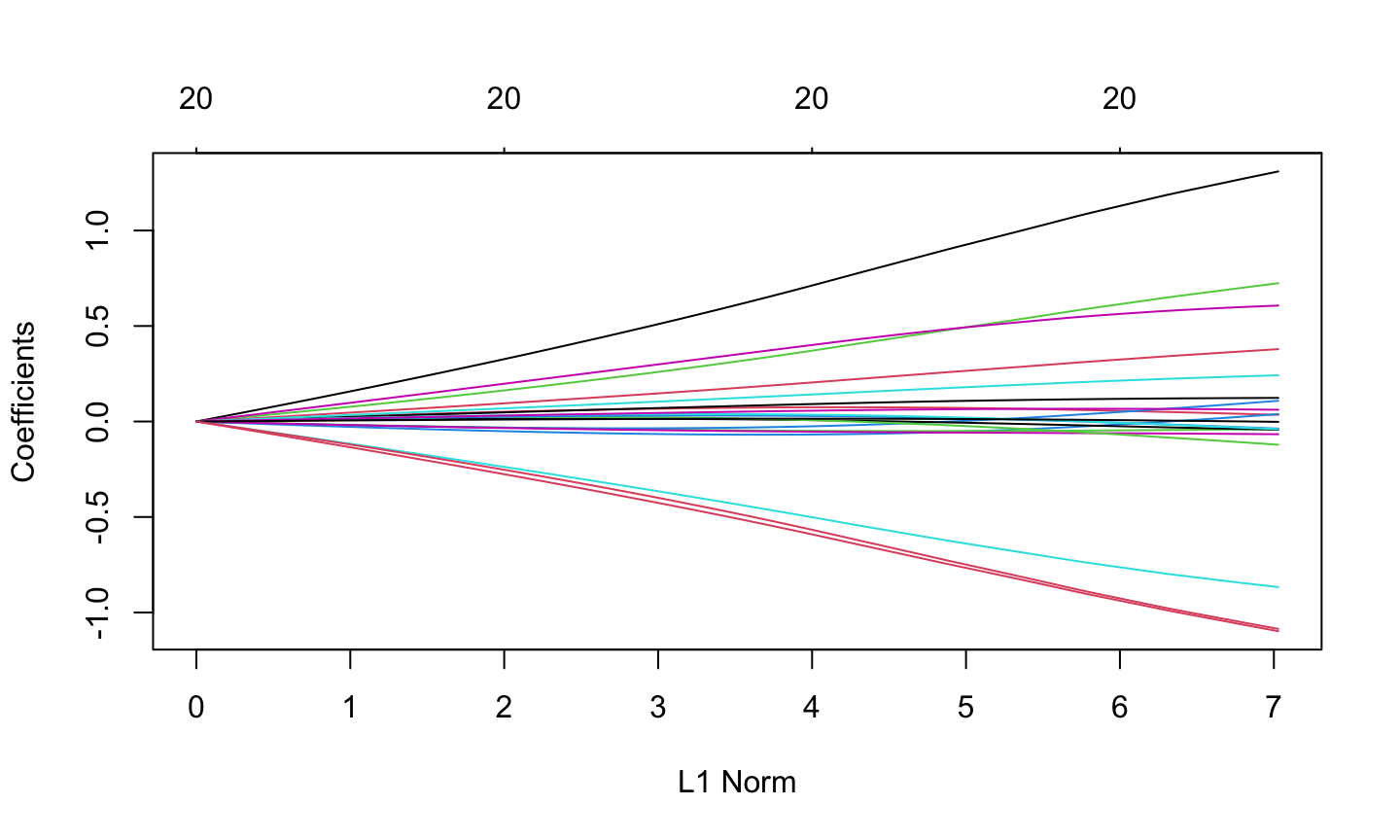
Package glmnet (Ridge)
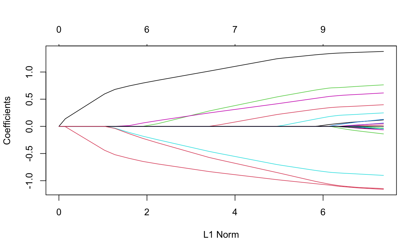
\[(1-\alpha)/2||\beta||_2^2 + \alpha ||\beta||_1\]
library(glmnet)
## Loading required package: Matrix
##
## Attaching package: 'Matrix'
## The following objects are masked from 'package:tidyr':
##
##     expand, pack, unpack
## Loaded glmnet 4.0-2
load("./data/QuickStartExample.RData")
fit1 = glmnet(x,y, alpha = 0)
plot(fit1)
Package glmnet (Lasso)
\[(1-\alpha)/2||\beta||_2^2 + \alpha ||\beta||_1\]
fit2 = glmnet(x,y, alpha = 1)
plot(fit2)
Summary
print(fit2)
##
## Call:  glmnet(x = x, y = y, alpha = 1)
##
##    Df  %Dev  Lambda
## 1   0  0.00 1.63100
## 2   2  5.53 1.48600
## 3   2 14.59 1.35400
## 4   2 22.11 1.23400
## 5   2 28.36 1.12400
## 6   2 33.54 1.02400
## 7   4 39.04 0.93320
## 8   5 45.60 0.85030
## 9   5 51.54 0.77470
## 10  6 57.35 0.70590
## 11  6 62.55 0.64320
## 12  6 66.87 0.58610
## 13  6 70.46 0.53400
## 14  6 73.44 0.48660
## 15  7 76.21 0.44330
## 16  7 78.57 0.40400
## 17  7 80.53 0.36810
## 18  7 82.15 0.33540
## 19  7 83.50 0.30560
## 20  7 84.62 0.27840
## 21  7 85.55 0.25370
## 22  7 86.33 0.23120
## 23  8 87.06 0.21060
## 24  8 87.69 0.19190
## 25  8 88.21 0.17490
## 26  8 88.65 0.15930
## 27  8 89.01 0.14520
## 28  8 89.31 0.13230
## 29  8 89.56 0.12050
## 30  8 89.76 0.10980
## 31  9 89.94 0.10010
## 32  9 90.10 0.09117
## 33  9 90.23 0.08307
## 34  9 90.34 0.07569
## 35 10 90.43 0.06897
## 36 11 90.53 0.06284
## 37 11 90.62 0.05726
## 38 12 90.70 0.05217
## 39 15 90.78 0.04754
## 40 16 90.86 0.04331
## 41 16 90.93 0.03947
## 42 16 90.98 0.03596
## 43 17 91.03 0.03277
## 44 17 91.07 0.02985
## 45 18 91.11 0.02720
## 46 18 91.14 0.02479
## 47 19 91.17 0.02258
## 48 19 91.20 0.02058
## 49 19 91.22 0.01875
## 50 19 91.24 0.01708
## 51 19 91.25 0.01557
## 52 19 91.26 0.01418
## 53 19 91.27 0.01292
## 54 19 91.28 0.01178
## 55 19 91.29 0.01073
## 56 19 91.29 0.00978
## 57 19 91.30 0.00891
## 58 19 91.30 0.00812
## 59 19 91.31 0.00739
## 60 19 91.31 0.00674
## 61 19 91.31 0.00614
## 62 20 91.31 0.00559
## 63 20 91.31 0.00510
## 64 20 91.31 0.00464
## 65 20 91.32 0.00423
## 66 20 91.32 0.00386
## 67 20 91.32 0.00351
Coefficients
coef(fit2, s=0.1)
## 21 x 1 sparse Matrix of class "dgCMatrix"
##                        1
## (Intercept)  0.150928072
## V1           1.320597195
## V2           .
## V3           0.675110234
## V4           .
## V5          -0.817411518
## V6           0.521436671
## V7           0.004829335
## V8           0.319415917
## V9           .
## V10          .
## V11          0.142498519
## V12          .
## V13          .
## V14         -1.059978702
## V15          .
## V16          .
## V17          .
## V18          .
## V19          .
## V20         -1.021873704
Prediction
nx = matrix(rnorm(10*20),10,20)
predict(fit2,newx=nx,s=c(0.1,0.05))
##                1          2
##  [1,] -2.9507090 -3.1022480
##  [2,]  2.9272360  2.9704542
##  [3,] -2.0321455 -2.0188869
##  [4,] -5.9819768 -6.3861583
##  [5,]  1.8483706  2.0048891
##  [6,]  1.8873977  1.9056910
##  [7,]  0.1925608  0.1935498
##  [8,] -3.6333085 -3.9299014
##  [9,] -0.4038197 -0.6322740
## [10,]  0.9123557  1.0305984
Determine \(\lambda\)
cvfit = cv.glmnet(x, y, alpha = 1)
plot(cvfit)
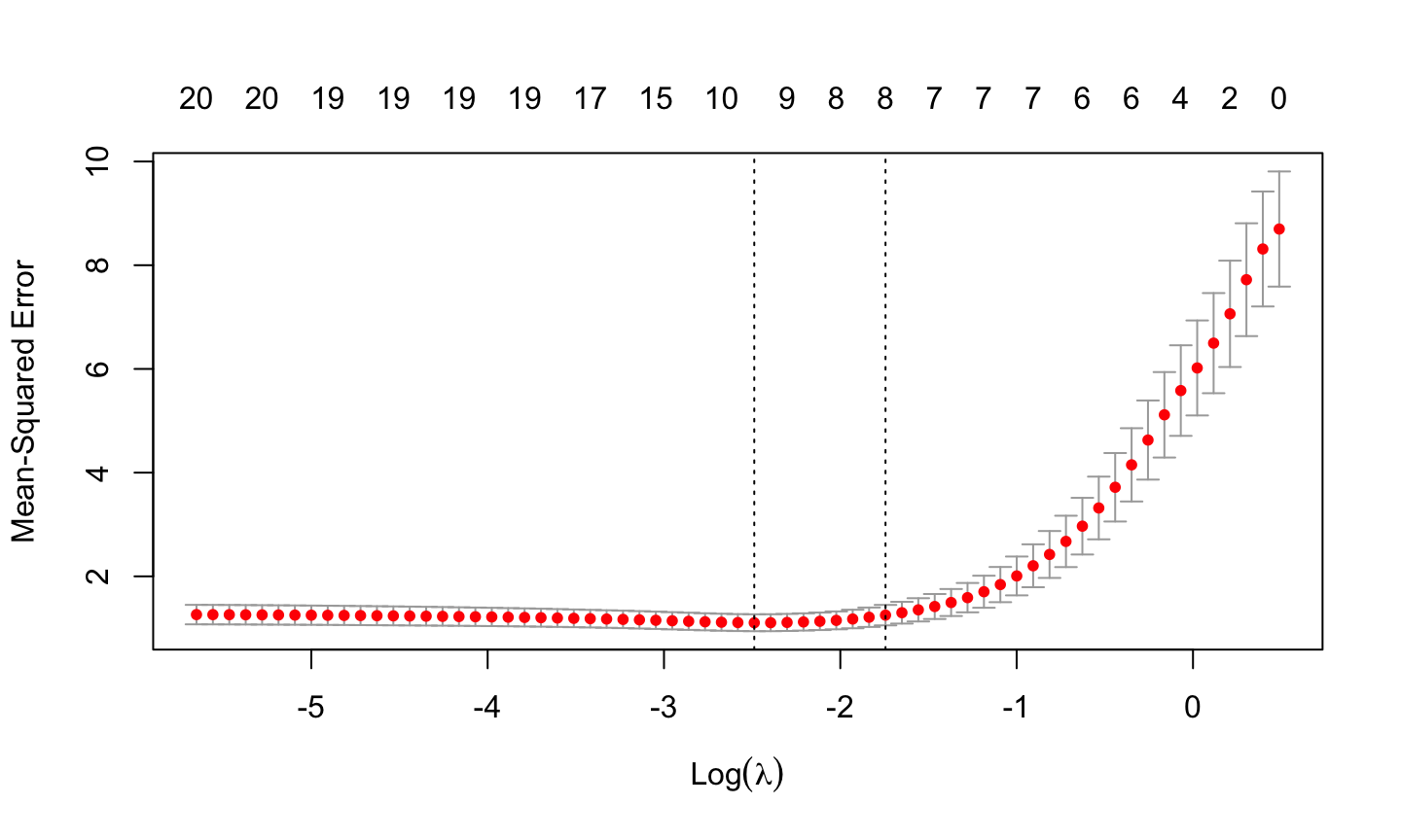
Selected \(\lambda\)
Value of \(\lambda\) that gives minimum mean cross-validated error
cvfit$lambda.min
## [1] 0.08307327
Value of \(\lambda\) that gives the most regularized model such that error is within one standard error of the minimum.
cvfit$lambda.1se
## [1] 0.1748613
More details
Friedman, J., Hastie, T., & Tibshirani, R. (2001). The elements of statistical learning (Vol. 1, No. 10). New York: Springer series in statistics.