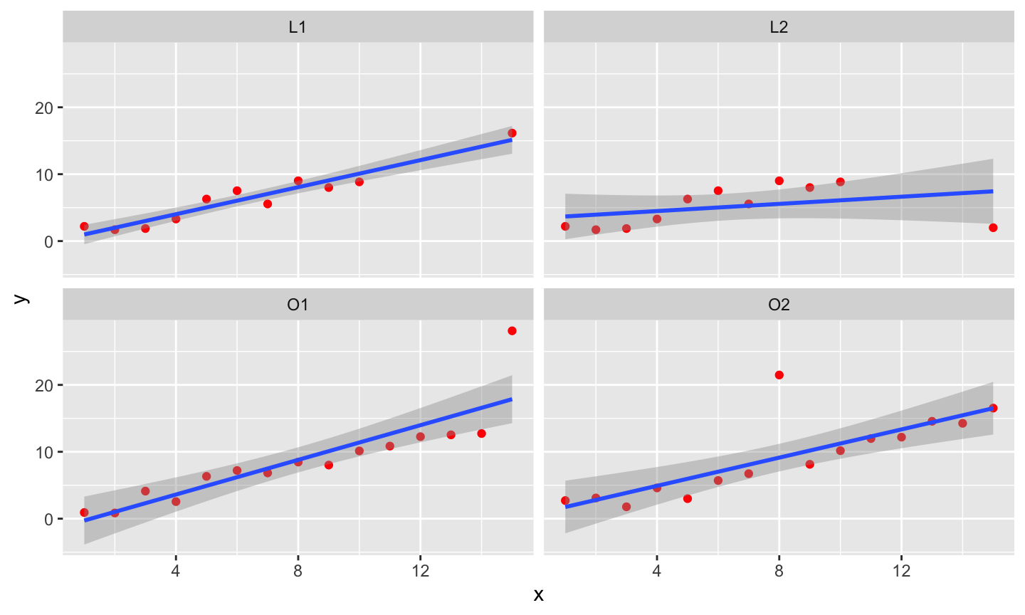
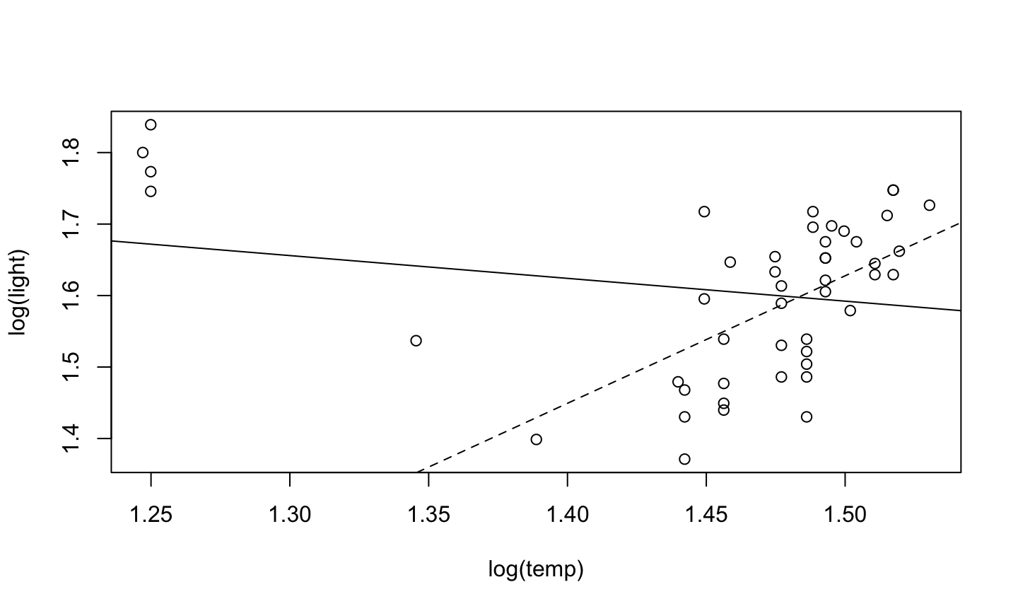
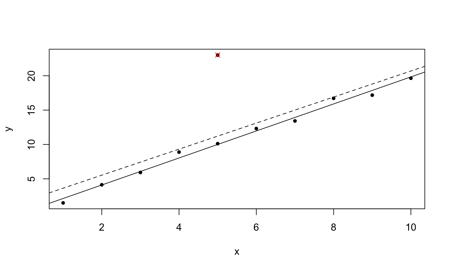
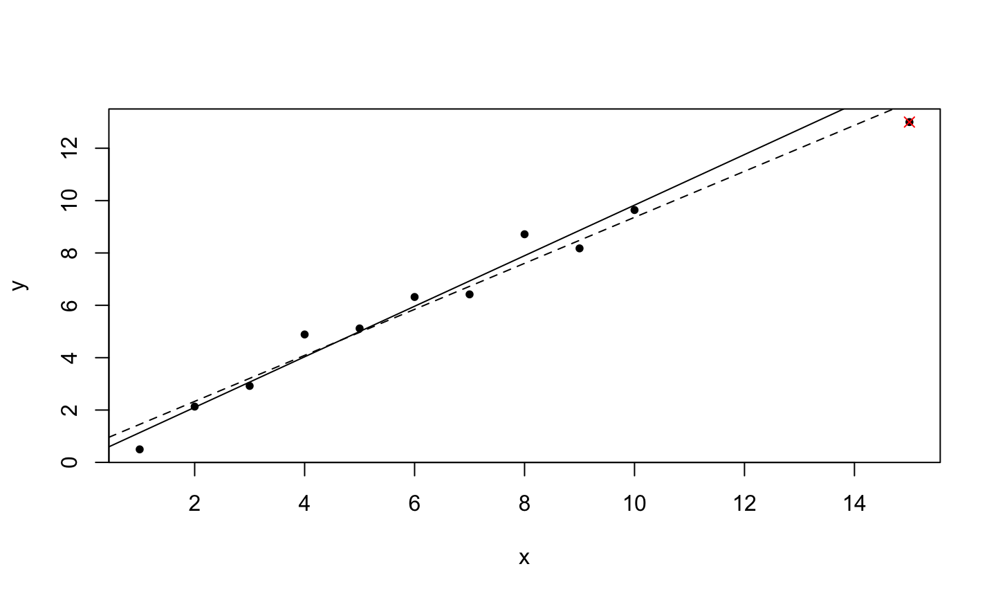
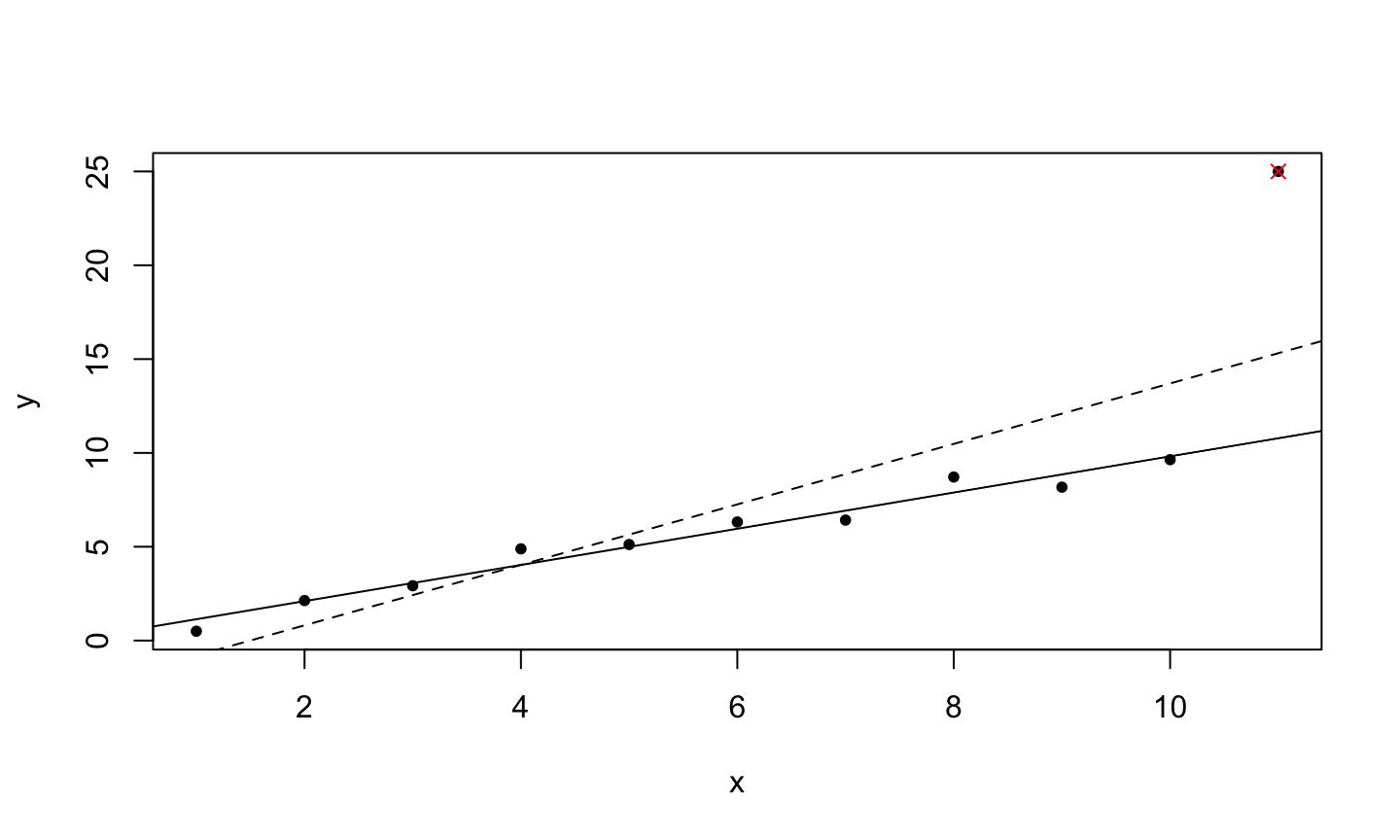
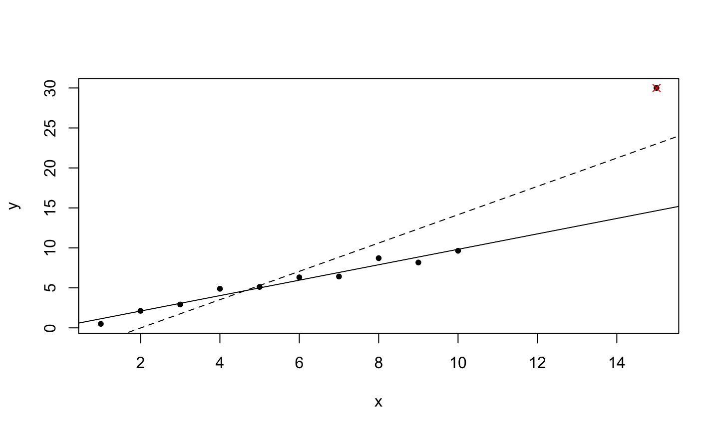
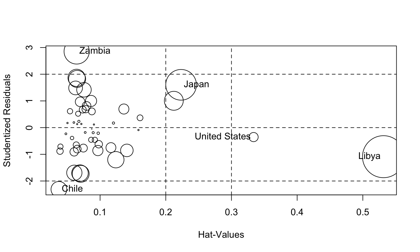
An implicit assumption made when fitting a regression model is that all observations should be equally reliable and have approximately equal role in determining the regression results and in influencing conclusions.

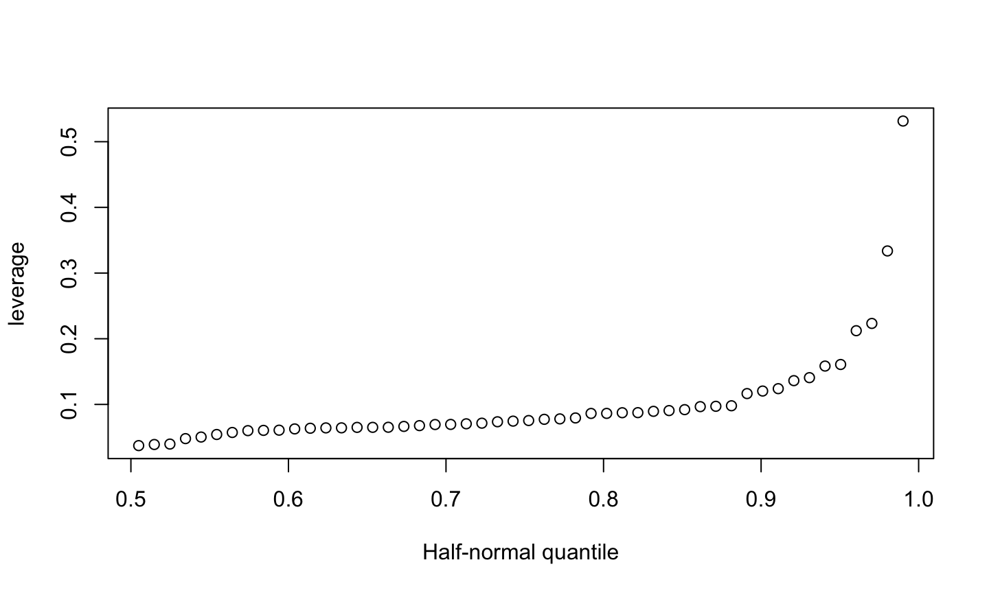
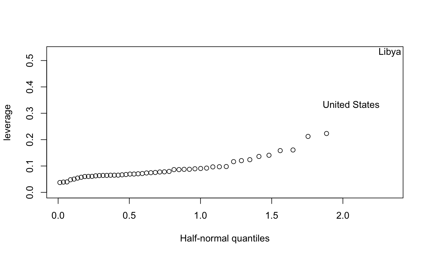
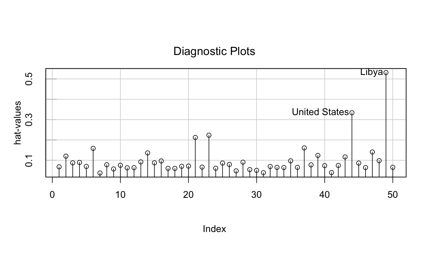
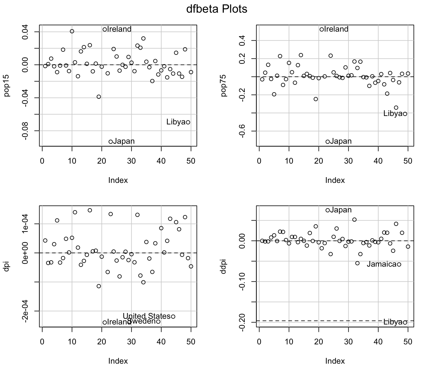
• A leverage point is an observation that is unusual in the predictor space.

• An outlier is an observation whose response does not match the pattern of the fitted model.

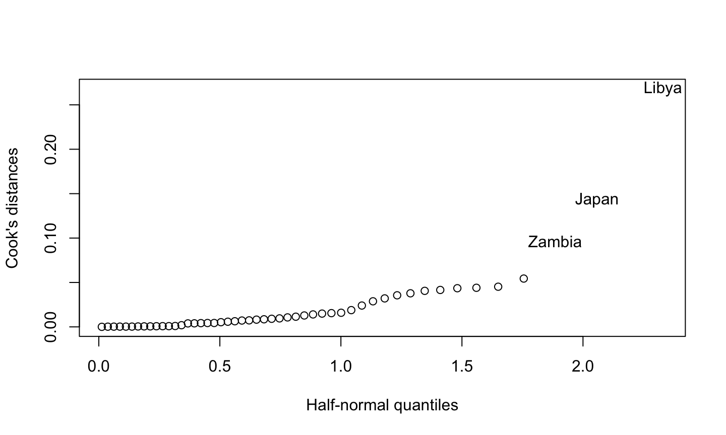
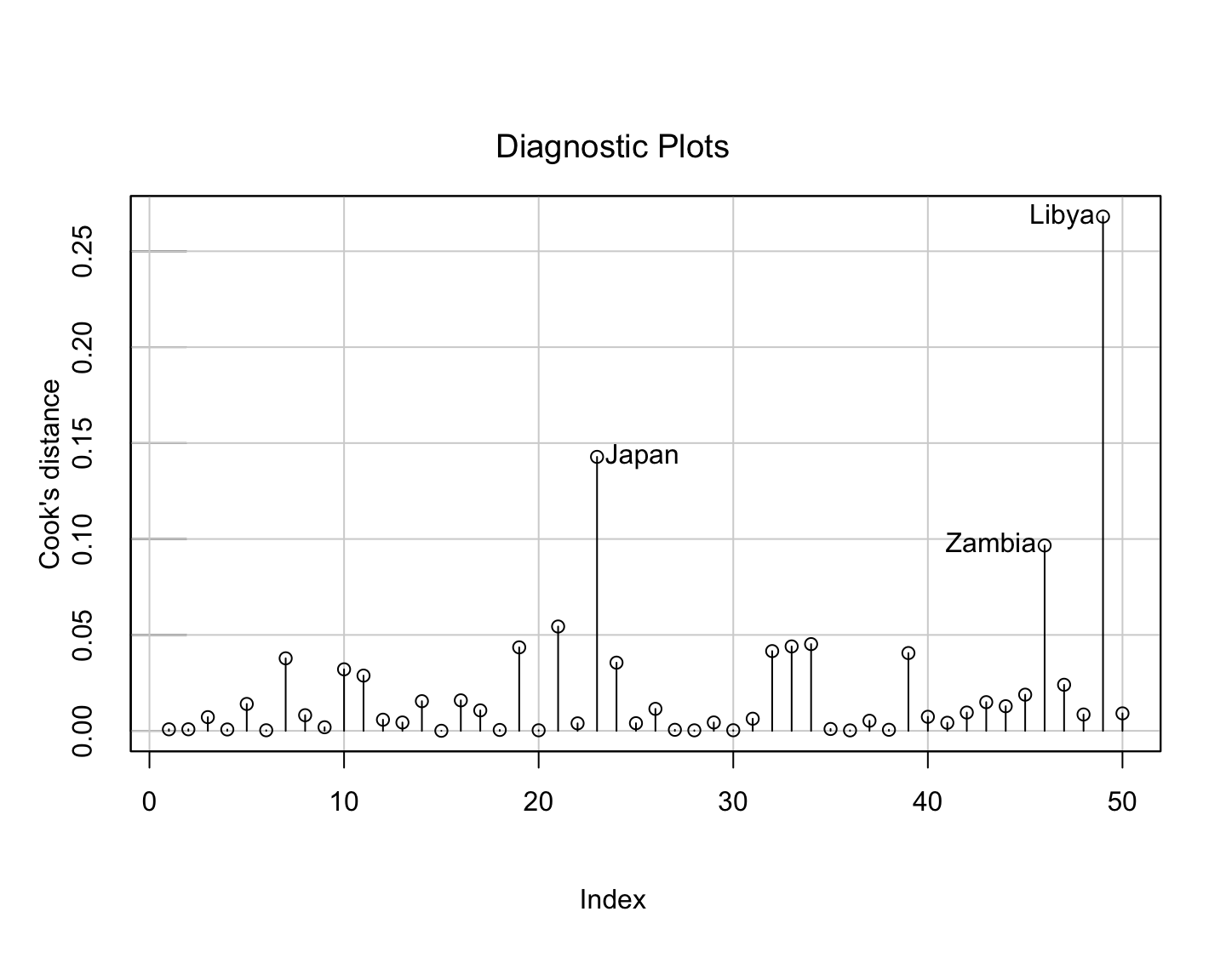
• An influential observation is one that causes a substantial change in the fitted model based on its inclusion or deletion from the model.

  • An influential observation is usually either a leverage point, an outlier, or a combination of the two.

• The fitted value \(\hat{y}_i\) is a linear combination of the observed \(Y\)

• \(h_{ii}\), the \(i\)th diagonal element of \(H\)

• \(h_{ii}\) is the weight of observation \(y_i\) in determining the fitted value \(\hat{y}_i\)

• The larger is \(h_{ii}\), the more important is \(y_i\) determining \(\hat{y}_i\)

• \(h_{ii}\) measures the role of the \(X\) values in determining how important \(y_i\) is in affecting \(\hat{y}_i\)

• \(h_{ii}\) is called the leverage value of the \(i\) th observation.
• Sometimes we write \(h_{ii}\) as \(h_i\)
• \(0\leq h_{ii}\leq 1\)
• \(\sum h_{ii} = p\)
• \(h_{ii}\) is a measure of distance between the \(X\) values for the \(i\)th observation from the mean of the \(X\) values of all \(n\) observations.

\[var(\hat{\epsilon}) = (I-H)\sigma^2\]

• \(var(\hat{\epsilon}_i) = (1-h_{ii})\sigma^2\)

• As \(h_{ii}\to 1\), \(\hat{y}_i\to y_i\)

The leverage values are the diagonal elements of the hat matrix \(H=X(X^T X)^{-1} X^T\).

The \(i\)th leverage value is given by \(h_i=H_{ii}\), the \(i\)th diagonal position of the hat matrix.

A half-normal plot of the leverage values can be used to identify observations with unusually high leverage.

• A half-normal plot compares the sorted data against the positive normal quantiles.

Rule of Thumb

• A leverage value \(h_i\) is usually considered large if it is more than twice as large as the mean leverage value.

The steps are:

• Sort the data: \(h_{[1]} \leq \dots h_{[n]}\) .
• Compute \(u_i=\phi^{-1} \left(\frac{n+i}{2n+1}\right)\).
• Plot \(h_{[i]}\) versus \(u_i\).

The leverage points are the points in the plot that diverge substantially from the rest of the data. If the half-normal plot is approximately a straight line of points, then there are no leverage points. If the half-normal plot looks like a hockey stick, then the points on the blade are leverage points.

y[15] = y[15] + 12

An index plot of the leverage values can also be used to identify leverage points.

• An index plot plots the statistic of an observation versus its observation number.
• You want to focus on observations where the statistics are large or small relative to the other values.

The car::infIndexPlot function can be used to generate index plots related to many influence-related statistics.

Consider the savings data frame in the faraway package that includes 5 savings-related variables in 50 countries averaged over the period 1960-1970. Fit the model regressing sr on the other four variables. Are there any leverage points?

data(savings, package = 'faraway')
lmod = lm(sr~.,data = savings)
n = nrow(savings)
u = (n+c(1:n))/(2*n+1)
plot(u, sort(hatvalues(lmod)), xlab = 'Half-normal quantile', ylab = 'leverage')

countries <- row.names(savings)
faraway::halfnorm(hatvalues(lmod), labs = countries, nlab = 2, ylab = "leverage")

car::infIndexPlot(lmod, vars = "hat")

An outlier is a point that does not fit the current model.

• An outlier is context specific! An outlier for one model may not be an outlier for a different model.

Leave-one-out statistics are statistics computed from the model fitted without the ith observation.

• \(\hat{\beta}_{(i)}\) is the vector of leave-one-out estimated coefficients.
• \(\hat{\sigma}_{(i)}\) is the leave-one-out estimate of the error standard deviation.
  
• \(\hat{y}_{(i)}\) is the leave-one-out fitted value for the ith observation.
• The \((i)\) means that these statistics were estimated for the model fitted without the ith observation.

If the leave-one-out residual (deleted residual) \(y_i-\hat{y}_{(i)}\) is large, then observation \(i\) is an outlier.

• The OLS residuals may not be suitable for identifying outliers since truly influential observations will pull the fitted model close to themselves, making the residual smaller.

When the model is correct and \(\epsilon∼N(0,\sigma^2 I)\), the externally studentized residual

\[t_i = \frac{y_i -\hat{y}_{(i)}}{\hat{\sigma}_{(i)}\sqrt{1+x_i^T\left(X_{(i)}^TX_{(i)} \right)^{-1}x_i}} \sim T_{n-p-1}.\] We can calculate a p-value to assess whether observation \(i\) is an outlier.

If performing multiple hypothesis tests at level \(\alpha\), the probability of making at least one type I error will be more than \(\alpha\). We must adjust the level of each test so that overall (familywise) type I error rate is satisfied. Suppose we want a level \(\alpha\) test for \(n\) tests, i.e., we want P(no type I errors in \(n\) tests)=\(1-\alpha\).

\[\begin{aligned} P(\text{no type I errors in }n \text{ tests}) = & P\left(\bigcap_{i=1}^n (\text{no type I error in test }i)\right)\\ = & 1- P\left(\bigcup_{i=1}^n (\text{type I error in test }i)\right)\\ \geq & 1- \sum_{i=1}^n P\left( \text{type I error in test }i\right)\\ =&1-n\alpha \end{aligned}\]

To get an overall level \(\alpha\) test, we should use the level \(\alpha/n\) in each of the individual tests.

This approach is known as the Bonferonni correction, and is used in many contexts to make proper simultaneous inference (not just for outliers or regression).

The Bonferonni correction is a very conservative method.

• It doesn’t reject \(H_0\) as often as it should.
• It gets more conservative as \(n\) gets larger.

A observation is considered an outlier if \(|t_i|\geq t_{n-p-1}^{\alpha/2n}\).

• Why do we divide by 2n and not just n?

stud <- rstudent(lmod)
max(abs(stud))

## [1] 2.853558

qt(1 - .05/(50*2), df = 44)

## [1] 3.525801

stud <- rstudent(lmod)
max(abs(stud))

## [1] 2.853558

qt(1 - .05/(50*2), df = 44)

## [1] 3.525801

alpha = 0.05
qt(1 - alpha/(nrow(lmod$model)*2), df = lmod$df.residual - 1) 

## [1] 3.525801

The studentized residuals are all within the expected range based on the quantile from the t distribution.

There is insufficient evidence to conclude that any observations are outliers.

The outlier test can be done almost automatically using the outlierTest function in the car package.

• Compare the Bonferonni p-value to the desired significance level.

car::outlierTest(lmod)

## No Studentized residuals with Bonferroni p < 0.05
## Largest |rstudent|:
##        rstudent unadjusted p-value Bonferroni p
## Zambia 2.853558          0.0065667      0.32833

car::infIndexPlot(lmod, vars = c("Studentized", "Bonf"))

• Two or more outliers next to each other can “hide” each other.
• If we fit a new model, we may get different or no outliers.
• If the error distribution is nonnormal, it is very reasonable to get large residuals.
• Individual outliers are less of a problem in larger datasets because they are not likely to have a large leverage.
• It is still good to identify the outliers.
• They probably won’t be an issue unless they occur in clusters.

Consider data of the log of the surface temperature and the log of the light intensity of 47 stars in the star cluster CYG OB1, which is in the direction of Cygnus.

The overall pattern of the data suggests a positive linear relationship, but the four stars create a major change!

Consider the model fit depending on whether the outliers are included in the model.

This is easy to visualize because we are only working in two dimensions—it gets much more difficult in higher dimensions.

• Robust regression would be the best approach here.

data(star, package = 'faraway')
lmod_w_outlier = lm(log(light) ~ log(temp), data = star)
plot(log(light) ~ log(temp), data = star)
abline(lmod_w_outlier)
lmod_wo_outlier = lm(log(light) ~ log(temp), data = star[log(star$temp)>1.3, ])
abline(lmod_wo_outlier,lty = 2)

An influential observation is one whose removal from the dataset would cause a large change in the fitted model.

• An influential observation is usually a leverage point, an outlier, or both.

In the plots below, an “additional” point is marked with a cross. The solid line is fit using the 10 original points and the dashed line is fit with original data and the added point.

abline(lm(y[-11]~x[-11]))

In the plots below, an “additional” point is marked with a cross. The solid line is fit using the 10 original points and the dashed line is fit with original data and the added point.

abline(lm(y[-11]~x[-11]))

The additional point is an outlier but has little effect on fit.

abline(lm(y[-11]~x[-11]))

abline(lm(y[-11]~x[-11]))

The additional point has large leverage but not an outlier or influential.

abline(lm(y[-11]~x[-11]))

abline(lm(y[-11]~x[-11]))

The additional point is outlier and influential.

abline(lm(y[-11]~x[-11]))

abline(lm(y[-11]~x[-11]))

High leverage: For sure. Outlier: Most probably. Influential: Yes.

Natural measures of influence are:

• \(\hat{y}_i - \hat{y}_{(i)}\), which will require us to look at vectors of length \(n\) for each observation \(i\).
  
• \(\text{DFBETA}_i=\hat{\beta} - \hat{\beta}_{(i)}\), which is a \(p\)-dimensional vector indicating how the estimated coefficients change when observations \(i\) is deleted from the data.

The Cook’s distance is a popular inferential tool because it reduces influence information to a single value for each observation.

The Cook’s distance for the ith observation is

\[D_i = \frac{(\hat{y} - \hat{y}_{(i)})^T(\hat{y} - \hat{y}_{(i)})}{p\hat{\sigma}^2} = \frac{1}{p}r_i^2\frac{h_i}{1-h_i}\]

Cook’s distance values can be obtained using the cooks.distance function.

A half-normal plot or index plot can be used.

lmod = lm(sr~.,data = savings)
cook <- cooks.distance(lmod)
countries = row.names(savings)
faraway::halfnorm(cook, n = 3, labs = countries, 
         ylab = "Cook's distances")

car::infIndexPlot(lmod, var = "Cook", id = list(n = 3))

How does the model fit change when we remove Libya from the data?

lmod2 <- lm(sr ~ ., data = savings, subset = (countries != "Libya"))
knitr::kable(car::compareCoefs(lmod, lmod2, print = F))

1: lm(formula = sr ~ ., data = savings) 2: lm(formula = sr ~ ., data = savings, subset = (countries != “Libya”))

          Model 1   Model 2

(Intercept) 28.57 24.52 SE 7.35 8.22

pop15 -0.461 -0.391 SE 0.145 0.158

pop75 -1.69 -1.28 SE 1.08 1.15

dpi -0.000337 -0.000319 SE 0.000931 0.000929

ddpi 0.410 0.610 SE 0.196 0.269

The coefficient for ddpi changed by about 50%, which is fairly large.

An index plot of the DFBETA statistics can be useful for assessing the direct impact of an observation on the estimated coefficients.

• DFBETA is the difference in the estimated coefficients when leaving out observation \(i\).
• DFBETAs is the DFBETA values divided by the leave-one-out estimate of the coefficient standard errors.

The car::dfBetaPlots or car::dfBetasPlots can be used to construct index plots of these statistics.

car::dfbetaPlots(lmod, id.n = 3)

An influence plot plots the studentized residuals versus the leverage values.

• This car::influencePlot function can be used to create this.
• Look for observations that have unusually large residuals, leverage values, and especially both.
• The circles are sized proportionally to the magnitude of the Cook’s distances

car::influencePlot(lmod)

##                  StudRes        Hat      CookD
## Chile         -2.3134295 0.03729796 0.03781324
## Japan          1.6032158 0.22330989 0.14281625
## United States -0.3546151 0.33368800 0.01284481
## Zambia         2.8535583 0.06433163 0.09663275
## Libya         -1.0893033 0.53145676 0.26807042

• If they’re data entry errors, correct the problem. If they can’t be fixed, remove them (they’re wrong, so they don’t tell us anything useful).

• Remove them if they’re not part of the population of interest (you are studying dogs, but this observation is a cat).

• Remove them because they break the model.

• This is a bad idea.

• Make sure to indicate that you removed them from the data set and explain why.

• THIS IS A BAD IDEA.

• An outlier/influential point for one model may not be for another.
• Examine the physical context—why did it happen?
• An outlier/influential point may be interesting in itself.
  • An outlier in a statistical analysis of credit card transactions may indicate fraud!
• This may suggest a better model.
• Use robust regression, which is not as affected by outliers/influential observations.
• Never automatically remove outliers/influential points!
• They provide important information that may otherwise be missed.
• Fit the model with and without the influential observation(s).
• Do your results substantively change?

• hatvalues extracts the leverage values from a fitted model.
• faraway::halfnorm constructs a half-normal plot
• infIndexPlot(lmod, vars = "hat") creates an index plot of the leverage values.

• car::outlierTest performs a Bonferonni outlier test
• infIndexPlot(lmod, vars = "Studentized") creates an index plot of the studentized residuals.

• cooks.distance extracts the Cook’s distances from a fitted model.
• faraway::halfnorm constructs a half-normal plot
• infIndexPlot(lmod, vars = "Cook") constructs an index plot of the Cook’s distances.
• plot(lmod, which = 4) constructs an index plot of the Cook’s statistics.
• car::dfBetaPlots and car::dfBetasPlots construct index plots of DFBETA and DFBETAS, respectively.
• car::influencePlot constructs an influence plot of the studentized residuals versus the leverage values.
• plot(lmod, which = 4) constructs an influence plot of the standardized residuals versus the leverage values.
• influence(lmod) computes a number of leave-one-out-related measures of observational influence.

Using the sat dataset in the faraway package, fit a model with the total SAT score as the response and expend, salary, ratio, and takers as predictors. Perform regression diagnostics on this model to answer the following questions.

• Check for leverage points.
• Check for outliers.
• Check for influential points.